Cells and Ranges in Excel

Cells and Ranges

Each cell is identified by its cell address, which is a combination of the column and row on which that cell is situated. A group of cells together are called ‘Range’.

When the group of cells you have selected are all together, it is called a Contiguous Range otherwise, it is called a Non-Contiguous Range. You can select the Non-Contiguous range by clicking on cells one-by-one with the CTRL key pressed.

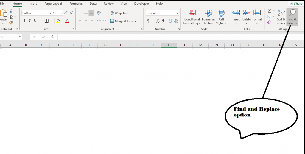
Find & Replace

The most commonly and frequently used features of Excel are Find & Replace. “Find” is used to search for a specified data value in an excel worksheet. It searches for all the possible values and marks them with different colors such that the user can easily recognize their position in the sheet.

Replace option is used to after the Find option, it alters the only data that meets the Find criteria the value with the one provided by the user.

If you want to find a particular value in an excel file -

• Under the Home tab ->Click on ‘Find’.

• A dialogue box appears. Write the name/value you want to search in your excel file.

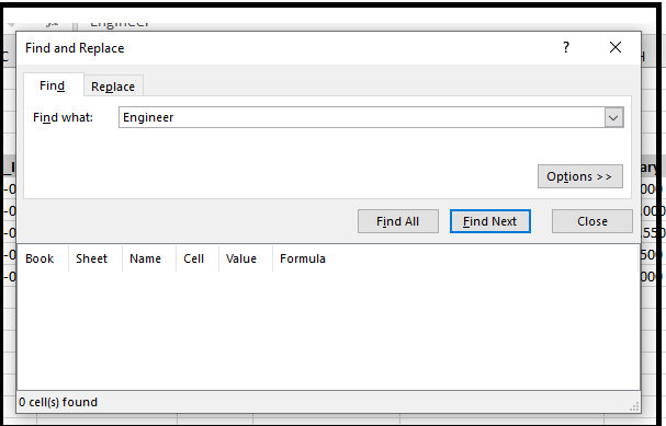
• Click on Find Next (it will show the next possible value that is present in the worksheet).

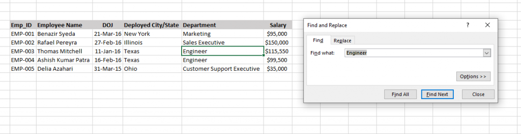
• Find All will give you all the locations of that value in the excel file.

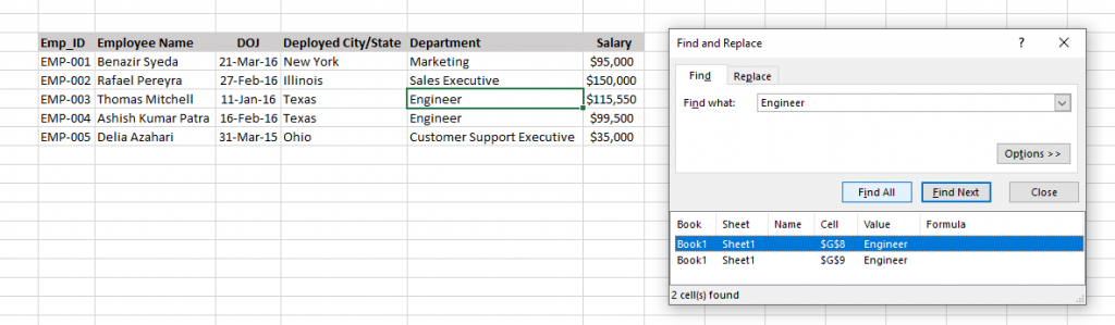
• A short-cut is CTRL+F

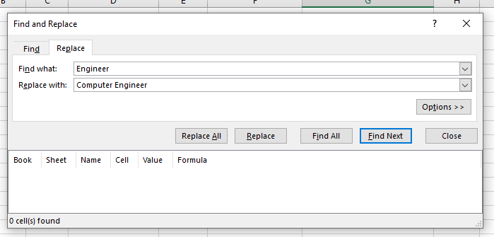
If you want to replace a particular value in an excel file -

• Click on ‘Replace’

• A dialog box appears. Write the name/value you want to replace

• Click on the Replace value option. It will replace or change only one value.

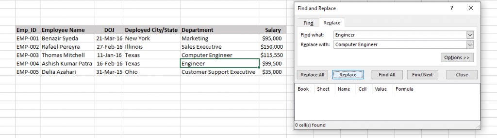
• Click Replace All for replacing that value in the entire tab.

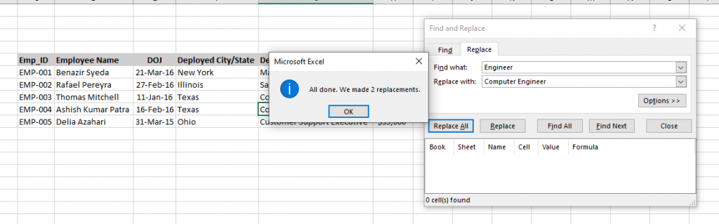
• A short-cut is CTRL +H

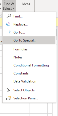
Go-to Special

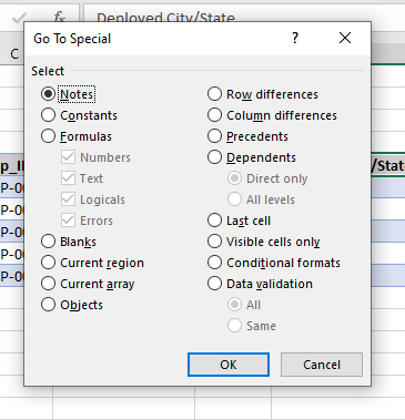
The Go-To Special function in Excel allows you to select all cells that meet certain criteria quickly. This command is used to identify specific cells – the ones which are used more have been listed below –

Comments - select only the cells that contain a cell comment

Constants - selects all nonempty cells that don’t contain formulas

Formulas - selects cells that contain formulas

Declaring Go-to special option

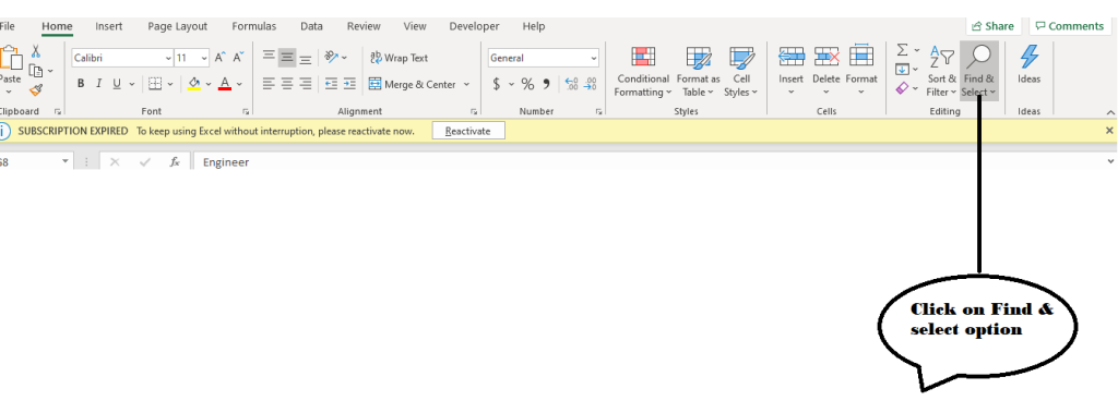
• Under the Home tab ->Click on ‘Find & Replace’.

• A dialog box appears. Click on Go-to special option.

• Go-to dialog box appears. The various options appear. Choose the appropriate once as per your requirement. Click on Ok

What is a Table?

Excel Table is a feature that can turn the range of cells/data into a Table format, which makes managing and analyzing data easier. It helps in managing the data in the table rows and columns independently from the data in other rows and columns.

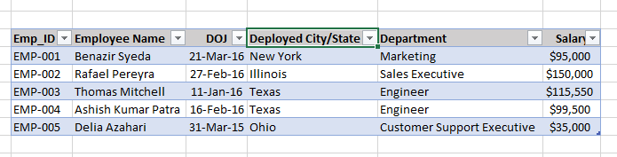
 In simple terms, it is a group of data – for ex: it maybe a list of students in a university and their details like age, roll no, marks, attendance together. It may be a list of items left in the stock at a supermarket and their quantities and prices mentioned.

You can use Table Feature to:

• Quickly Calculate and Display the Data Sets
• Use Structured References
• Quickly Inserts or Deletes Table Rows & Columns
• Formatting Table Quickly etc.

Declaring a dataset as a Table

• Open or go to the sheet which has that dataset.

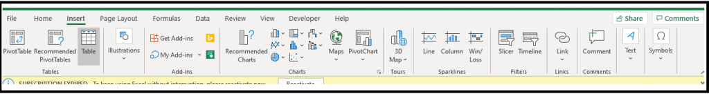
• Go to ‘Insert’ group and click on ‘Table’

• A dialog box appears wherein your cell range has been selected.

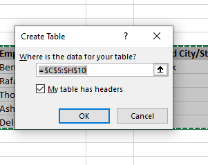
• Excel will select the dataset and just press ‘OK’ to make it a table. Your selected data will be converted to a table.

Advantages of declaring a dataset a Table

• Different Format options available to color the table
• Auto-populates the formulas on adding a formula to one cell
• You can calculate a lot of metrics by clicking on ‘Total’ in the ‘Design’ tab which appears when you have clicked on any cell in the said table
• Excel automatically adds filters to a table thus making it easier to sort and filter data
• Headers are always visible so that you do not need to freeze window pains
• Auto-updates charts i.e., whenever you add new rows or change data, excel will automatically update the charts – please do remember that if you change the data, the charts will get updated then also irrespective excel knows your dataset is a table or just a dataset

Freeze Panes

This feature in Microsoft Excel allows locking specific rows/columns to keep them always visible scrolling horizontally or vertically through the worksheet. A portion of the sheet is freeze to keep it visible while you scroll through the rest of the sheet.

 It is very useful when you have a large table of data in Excel or in checking out the data in other parts of your worksheet without losing the headers or labels.

Different Freeze Panes Options

• Freeze Rows
• Freeze Columns
• Freeze Current Selection
• Unfreeze panes

Steps for applying freezing panes are as follows:

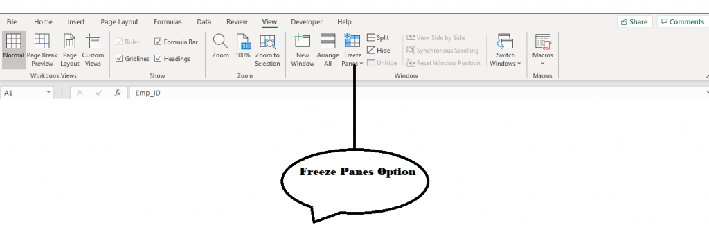
1. Under the ribbon tab, click on Freeze Panes option.

• Freeze Pane option box appears, choose the desired option as here we want to freeze the top row.

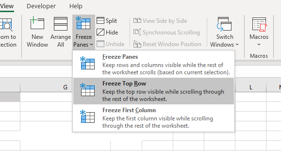
• The top row is now visible if you scroll down to the lowest cell.

• Similarly, you can freeze the column of the excel sheet.

Note: Freeze Panes cannot be used when editing any cell. You can only freeze Rows at the top and Columns on the left side of the active worksheet.

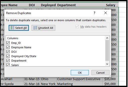
Remove Duplicates

Excel provides the inbuilt feature to remove the duplicates data in a worksheet. It deletes the duplicate rows from the sheet. You can even pick which column should be checked for duplicate information. This improves the readability and uniqueness of the data. The user has not to manually find and delete the repeated data.

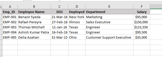
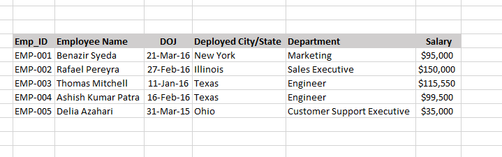
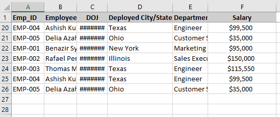
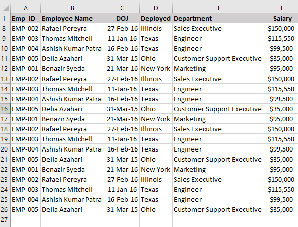
Create a list of Emp id, names, DOJ, State, Department and Salary in column A, B, C, D, E, F.

1. Repeat some names in your worksheet. Select the range of cells from where you want to remove the duplicates.

• Go to ‘Data’ ->Click on ‘Remove Duplicates’.

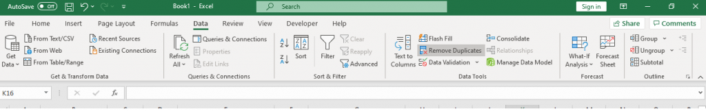
• Click on ‘OK’ to proceed

• A dialog appears, indicating the total values that have been removed and the total unique values present in the worksheet.

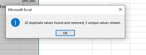
• The sheet will be left with only the unique set of values.