Graphs in D3.js
Graphs in D3.js
A graph can be described as a two-dimensional structure. It is also defined as a flat structure. A graph structure contains the coordinate space in which the value of x = 0, and y = 0 that tends from the bottom left side. In mathematics, the Cartesian Coordinate Space Graph containing x coordinate tends from left to right, and y coordinate tends from bottom to top. It means if you want to draw a circle with the help of x and y coordinates that contains value (20, 20), then you required to go 20 pixels from bottom left to right and 20 pixels upside.
SVG Coordinate space
In the SVG coordinate space, the coordinate x tends from left to right side, and y tends from bottom to top side. The working functionality of coordinate space is similar as mathematical graph coordinates, excluding two essential properties. They are-
- If the coordinate space x = 0 and y = 0, then the coordinate are situated at the top left side of the graphs.
- The SVG coordinate space contains the y coordinate tends from the top side to the bottom side.
SVG Coordinate Space of Graph
If you are going to draw a circle with the help of x, which contains 40 and y coordinate contains 40 value, then you need to go 40 units from bottom left to right and then go 40 units upside as explained in the below code:
var svgContainer = d3
.select(“body”)
      .append(“svg”)
      .attr(“width”, 300)
      .attr(“height”, 300);
In the above-given code, we have the SVG elements of a graph, where x = 300 width and y = 300 height. As you know that the x and y zero (origin) coordinates always lie on the top left. In D3.js, the y coordinate of the graph tends from top to bottom. You can determine the SVG elements, as shown in the below code:
var svgContainer = d3
.select(“body”) .append(“svg”)
      .attr(“width”, 300)
      .attr(“height”, 300)\
       .style(“border”, “2px solid blue”);
Line Graph
A line graph is used to depict the significance of a variable over time. The line graph measures the two variables, and each variable is assigned with its axis. A line graph consists of both types of the axis, such as horizontal and vertical.
Here, we have an example of a graph representing a CSV file (Comma-separate values), which shows the Indian Population growth from 2006 to 2020.
Now, we create a CSV file to define population. It is determined in below code:
Year, Population
2006, 42
2008, 48
2010, 52
2012, 53
2014, 55
2016, 57
2018, 59
2020, 62
Now, we save the file. Here, some steps are mentioned below to create a line graph:
Step 1: Adding the styles- In the first step, you can add any style in the line class with the help of the below code.
.line
{
            fill: none;
            stroke: brown;
            stroke-width: 8px;
}
Step 2: Variable Defining- You are required to define the variable with the help of SVG attributes as shown in below code:
var margin = {top: 25, right: 25, bottom: 35, left: 55},
width = 950 – margin.left – margin.right,
height = 400 – margin.top – margin.bottom;
In above code, the margins (top, bottom, left, right) determine the positioning point of the graph.
Step 3: Line Defining- In this step, you are required to create a new line with the help of d3.line() function. It is explained in the below code:
var valueline = d3.line()
.x(function (d) {   return  x(d.year);   })
.y(function (d) {   return  y(d.population);   });
Here, x represents the data of x-axis and population represents the data of y-axis.
Step 4: Affix the SVG attributes- Now, you need to affix the attributes with the help of append() method as represented in the below code:
var svg = d3.select(“body”).append(“svg”)
        .attr(“width”, width + margin.left + margin.right)
        .attr(“height”, height + margin.top + margin.bottom)
     .append(“g”) .attr(“transform”, “translate(“   + margin.left  + “ , ”  +  margin.top + ”)” );
The above code represents the affixing of the group elements and enforces the transformation.
Step 5: Data Reading- You can read data from the data collection (data.csv) as given in the below code:
d3.csv (“data csv” , function (error, data)
{
            if (error) throw error;
}
If the code doesn’t have the data.csv, then it displays an error.
Step 6: Data Formatting- For data formatting, you can use the below-given code:
data.foreach(function(d)
{
            d.year = d.year;
            d.poplulation = +d.population;
});
The above code assures that all the values extracted from the CSV file are correctly formatted and set. Here, we have two rows, one for ’year’ and second for ‘population.’ The function d helps to extract the value of population and year in one row at a time.
Step 7: Scale Range Setting- After the data formation, you are required to set the scale range for both coordinates (x and y). It is explained in the below code:
x.domain(d3.extent(data, function(d) {  return d.year;   } ));
y.domain([0,  d3.max(data, function(d) {  return d.population;   } )]);
Step 8: Appending the Path- In this step, you need to affix data and path by using append() method as represented in the below code:
svg.append (“path”) .data([data])
      .attr(“class”, “line”)
      .attr(“d”, valueline);
Step 9: Add the x-axis- Now, the code requires the adding of coordinates. The addition of x-axis to the group is presented in the below code:
svg.append (“g”)
      .attr(“transform”, “translate(0, “   +  height  +   ”) ”)
      .call(d3.axisBottom(x));
Step 10: Add the y-axis- The addition of y-axis to the group is described in the below code:
svg.append(“g”)
 .call(d3.axisLeft(y));
Step 11: Complete Example- In this step, we have a proper executable program code explained in code blocks. Now, you need to create a simple HTML file named linegraph.html and perform the below mentioned changes:
<!DOCTYPE html>
<html>
<head>
<script type = "text/javascript" src = "https://d3js.org/d3.v4.min.js"></script>
<style>
         .line {
            fill: none;
            stroke: green;
            stroke-width: 8px;
         }
</style>
</head>
<body>
<script>
 // set the dimensions and margins of the graph
 var margin = {top: 25, right: 25, bottom: 35, left: 55},
 width = 950 - margin.left - margin.right,
 height = 400 - margin.top - margin.bottom;
 var x = d3.scaleTime().range([0, width]);                  // set the ranges
 var y = d3.scaleLinear().range([height, 0]);
 var valueline = d3.line()                                             // define the line
    .x(function(d) { return x(d.year); })
    .y(function(d) { return y(d.population); });
 // append the svg obgect to the body of the page
 // appends a 'group' element to 'svg'
 // moves the 'group' element to the top left margin
 var svg = d3.select("body").append("svg")
    .attr("width", width + margin.left + margin.right)
    .attr("height", height + margin.top + margin.bottom)
    .append("g").attr("transform",
    |"translate(" + margin.left + "," + margin.top + ")");
 d3.csv("data.csv", function(error, data) {                        // Get the data
if (error) throw error;
data.forEach(function(d) {                                              // format the data
    d.year = d.year;
    d.population = +d.population;
    });
   // Scale the range of the data
    x.domain(d3.extent(data, function(d) { return d.year; }));
    y.domain([0, d3.max(data, function(d) { return d.population; })]);
    svg.append("path")                                                  // Add the valueline path.
    .data([data])
    .attr("class", "line")
    .attr("d", valueline);
    svg.append("g")                                                        // Add the X Axis
    .attr("transform", "translate(0," + height + ")")
    .call(d3.axisBottom(x));
    svg.append("g")                                                        // Add the Y Axis
    .call(d3.axisLeft(y));
 });
</script>
</body>
</html>
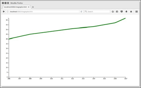
Output
After the successful execution of the code, you will get the following output: