How to create drop down in excel?
How to create drop down in excel?
Drop-down lists are mostly used to facilitate data entry operations. They are commonly used in interactive websites or applications. Microsoft has expanded his Excel's data validation feature to make manageable lists with the help of drop-down feature within your worksheets. Microsoft users use this feature to limit the selection choice, create a list of valid choices that can be used to select the specified field and to control the visibility list. This feature is very intuitive for the user and is an excellent approach to provide the user with a pre-defined list from where he can select his own options. This feature also enables the efficiency of data entry and reduces the risk of typing errors. In Excel, they are mostly used in user forms or in creating Excel dashboards.
There are three kinds of dropdown list that can be created in Microsoft Excel:
- Simple drop-down Lists
- Dynamic drop-down Lists
- Dependent drop-down Lists
Simple drop-down Lists
Simple drop-down lists are useful for creating fields that need certain information and require long or complex data where you want to control the user responses. To create a simple drop-drop list follow the given steps:
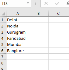
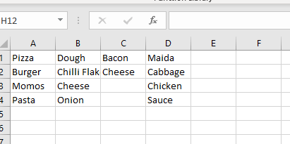
- In the excel sheet, type all the required data that you want to list down in your drop-down list.
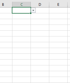
- Place your cursor where you want to display the drop-down list. For an instance, here we have selected the C1 cell.

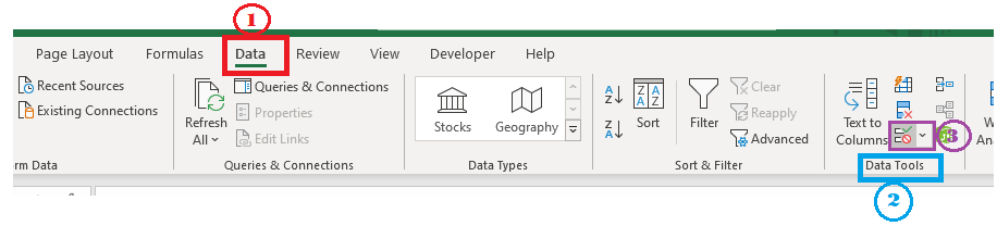
- Click on Data ribbon toolbar-> select data validation.

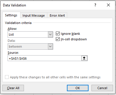
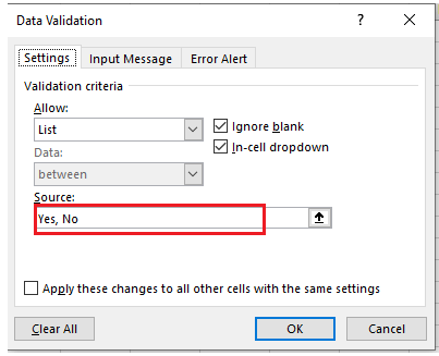
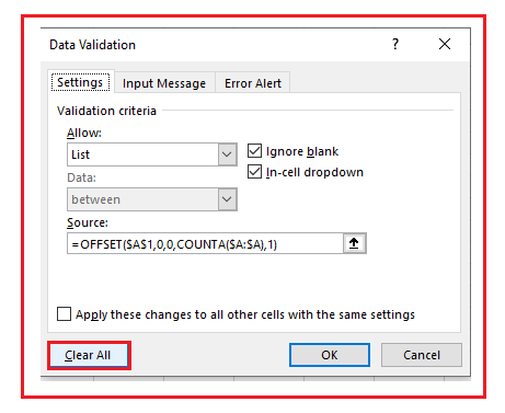
- The data validation dialog box will appear. The validation criteria have two parameters i.e., Allow and source.
- In the allow parameter select the require type i.e list.
- the source parameter is used to mention the data range (data you want to display in the drop-down list).
- Click on OK
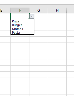
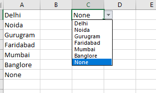
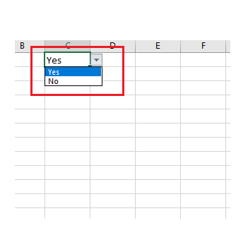
- You will notice that the drop-down list has been created in the selected cell.
- One can directly type the values in the source data instead of writing them separately in excel and then latterly using the reference range.
- Result for the above source data is given below.
Dynamic drop-down Lists
Dynamic drop-down lists are very convenient to use as it allows the user to select the data without making any changes to the source. It is similar to the simple drop-down validation. However, when you make any amendments in the source data t, the dynamic drop-down list changes automatically to accommodate that action, whereas in the case of simple drop-down list you have to manually refresh the drop-down validation feature. Hence, you need not to amend or refresh the drop-down data validation every time to get the updated drop-down list.
It is created with the help of Excel function. Below are the given steps to create a dynamic drop-down list:
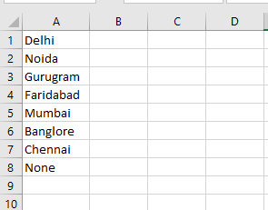
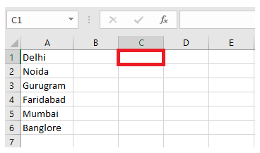
- In the excel sheet, type all the required data that you want to list down in your drop-down list.
- Place your cursor to the cell where you want to display the drop-down list. For an instance, here we have selected the C1 cell.
- Click on Data ribbon toolbar-> select data validation.

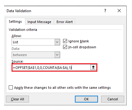
- The data validation dialog box will appear. The validation criteria have two parameters i.e., Allow and source.
- In the allow parameter select the require type i.e list.
- In the source parameter mention your formula to fetch data range: =OFFSET($A$1,0,0,COUNTA($A:$A),1)
- Click on OK
Explanation of Formula: The excel offset function consists of 5 parameters. Reference: Sheet1!$A$1, rows set to offset: 0, columns set to offset: 0, height: COUNTA(Sheet1!$A:$A) and width: 1. COUNTA function is used to count the number of values in column A on Sheet1 that are not empty.
Whenever the user adds any data in the excel list the COUNTA automatically increases. Thus, expanding the range returned by the OFFSET function and updating the drop-down list.
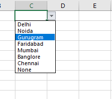
- You will notice that the drop-down list has been created in the selected cell.
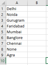
- Now, let’s add another a new item to the end of the excel list in order to check whether the list will be updated automatically or not.
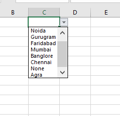
- You will notice that the new item has been automatically updated in the drop-down list as shown below.
Steps to remove drop-down list from Excel
- Select the cell where you have placed the drop-down list. Unlike here we have selected C1 cell.
- Click on Data ribbon toolbar-> select data validation.
- The data validation dialog box appears.
- At the below of the dialogue box, you will find Clear All option. Click on the option.
- Click on OK
- You will notice that the drop-down list has been removed from the Excel sheet.
Dependent drop-down Lists
In Excel the Dependent drop-down list are the replica of submenus in office applications. The data in the main drop-down list further displays another set of options categorically. This feature enables the user to select a category from the main menu drop-down list (such as Beverages), then it shows all the products related to the main product from the submenu. Thus, it adds on an advantage and is very helpful for dividing the products into handy categories (commonly used in ordering and inventory purposes). That is why the retails and wholesale companies prefer to excel dependent drop-down list to manage their product lines.
Following are the steps to execute the dependent drop-down list in your excel sheet:
- In the excel sheet, type all the required data along with their subcategories that you want to list down in your drop-down list.
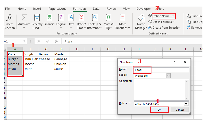
- Specify you the define name group for specific data range.
- Select the data range.
- Under the formula tab ->Defined Names-> select Define Name
- A dialog box will appear. Specify your name and click on Ok.
- Select the cell where you want to display the drop-down list. Click on Data ribbon toolbar-> select data validation.

- A dialog box will appear. The validation criteria have two parameters i.e., Allow and source.
- In the allow box, select the list data type.
- In the source parameter type =Food
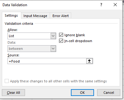
- You will notice in F1 cell, your dependent drop-down list has been created.