K-means clustering Algorithm
Introduction to K-means clustering
K-mean clustering comes under the unsupervised based learning, is a process of splitting an unlabeled dataset into the clusters based on some similarity patterns present in the data. Given a set of m nos. of the data item with some certain features and values, the main goal is to classify similar data patterns into k no. of clusters.
The datapoints are allocated to each cluster in such a way that the summation of the squared distance among the datapoints and the centroid is minimum. Lesser the variations in the clusters more would be the similar datapoints enclosed in a cluster.
Working of K-means clustering
Step 1: First, identify k no.of a cluster.
Step 2: Next, classify k no. of data patterns and allocate each of them to a particular cluster.
Step 3: Compute centroids of each cluster by calculating the mean of all the datapoints contained in a cluster.
Step 4: Keep iterating the steps until an optimal centroid is found.
Implementation in Python
As usual, our first step is to import all the three essential libraries i.e., numpy to use mathematics, matplotlib to plot nice charts and pandas to import and manage datasets more easily, as done in the preceding models.
# Import the libraries
import numpy as np
import matplotlib.pyplot as plt
import pandas as pd
After importing the libraries, the next step is to import the dataset with the help of the pandas library as a data frame. Here we will import the dataset of a mall.
# Import the dataset
dataset =pd.read_csv('Mall_Customers.csv')
Output:
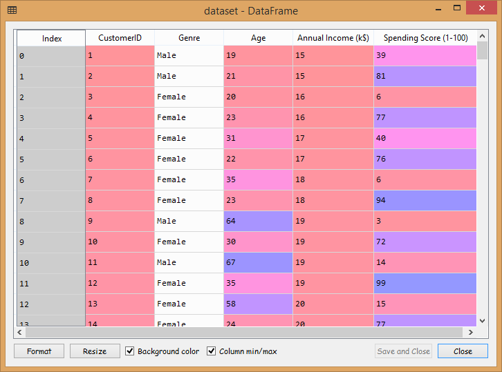
The mall dataset contains the information of the clients that have subscribed to the membership card of the mall of a particular city. At the time of subscription, the clients provided their details such as Gender, Age, and Annual income. As the user purchases from the mall with the same card, so the mall keeps each user purchase history, and that's how we get the last column i.e., Spending Score (1-100), which is computed by the mall for each of its clients based on some criteria.
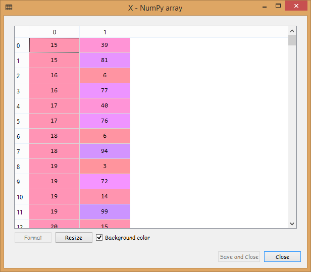
Now we will segment the clients into different groups based on Annual Income and Spending Score. Since we have no idea about how many segments of clients would be there, and we have no answer to this question, it is particularly a clustering problem. So, we will begin with a k-means clustering algorithm to find out what those clusters of clients might be, and for that, we will build an array comprising of two columns that we are interested in i.e., the annual income which is at 3rd index and spending score at 4th index.
X = dataset.iloc[:, [3, 4]].values
The array can be visualized by clicking on X at the variable explorer pane, and we will get the following output;
Output:
Now that we are done with importing the dataset, we will specifically start with k-means clustering. In k-means clustering, we are required to choose the no. of clusters, but here as we are not aware of how many no. of clusters of clients to look for. So, we will find an optimal no of clustering for our problem by incorporating the elbow method.
We will first import the KMeans class from scikit learn, followed by plotting the elbow method graph. And for that, we will compute within cluster sum of squares for ten different no of clusters. Since we are going to have ten different iterations, we are going to use for loop to create a list of ten different within cluster sum of squares for the ten no. of clusters.
We will start by initializing the list called wcss, and then the loop is started for i in range 1 to 11, such that 1 bound is included and 11 bound is excluded because we want 10 wcss. In each iteration of this loop, we will do two things:
- Firstly we will fit the k-means algorithm to our data X, for that we will create an object kmeans of class KMeans and within the class, we are going to pass several parameters;
- n_clusters called as no. of clusters
- init, which is the random initialization method. Since we don’t want to fall into the random initialization trap, we have chosen a very powerful method k-means++ instead of random.
- max_iter, which is termed as a maximum no. of iterations that defines the final cluster when the k-means algorithm is running. Here we have selected the default value i.e., 300.
- n_init, that is the no. of times the k-means algorithm will run with different initial centroids. The default value i.e., 10, is chosen by us.
- random_state, which fixes all the random factors of the k-means process.
Now that we are done making the k-means algorithm, we will now fit it to the data X using the fit() method.
- Secondly, we will compute the within cluster sum of squares independent to the wcss list. There is another name for within cluster sum of squares called as inertia. The scikit learn library has provided us with an inertia attribute that will compute within cluster sum of squares.
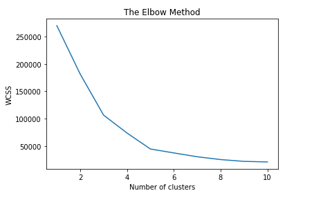
Next, we will plot the elbow method graph, and for that, we will pass the X-axis values that are in range (1,11) because we want 10 no. of clusters and the Y-axis values, which is wcss. To the graph, we have named the title as “The Elbow Method”, the xlabel as “Number of clusters” and the ylabel as “wcss." To display the graph, plt.show() method is used.
# Use the elbow method to find the optimal number of clusters
 from sklearn.cluster import KMeans
 wcss = []
 for i in range(1, 11):
 kmeans = KMeans(n_clusters= i, init = 'k-means++', max_iter=300, n_init=10, random_state = 0)
kmeans.fit(X)
wcss.append(kmeans.inertia_)
 plt.plot(range(1, 11), wcss)
 plt.title('The Elbow Method')
 plt.xlabel('Number of clusters')
 plt.ylabel('WCSS')
 plt.show()
Output:
Upon execution of the above code, we can clearly see that we get five optimal clusters which can be seen from the elbow chart given below.
Now that we have the right no. of clusters, we are ready to start our next step that is applying the K-means algorithm to the dataset X with the exact no. of clusters. This step is similar to the step we performed in the previous step inside the loop. The only difference is that now we will take n_cluster equals to 5, keeping the rest input parameters untouched.
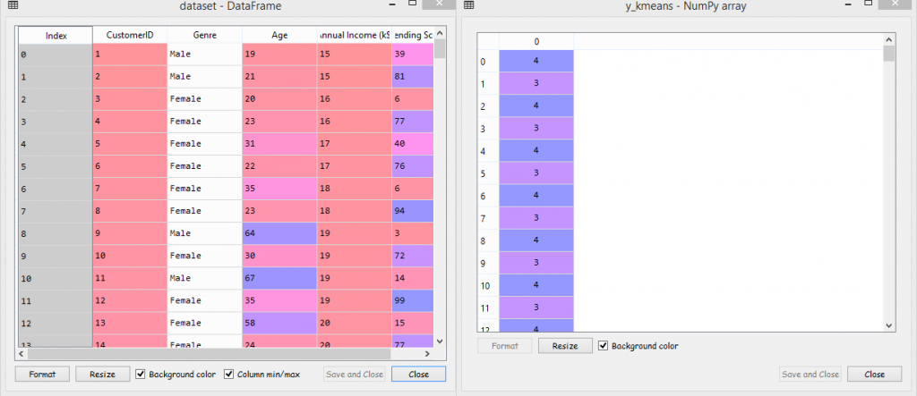
Next, we will fit the kmeans to the dataset X, and for that, we will use the fit_predict method as for every single client of our dataset it is going to tell us a cluster to which the client belongs by returning its cluster no into a single vector that we have named as y_kmeans.
# Fit K-Means to the dataset
 kmeans = KMeans(n_clusters = 5, init = 'k-means++', max_iter=300, n_init=10, random_state = 0)
 y_kmeans = kmeans.fit_predict(X)
After executing the above two lines, if we go to Variable explorer, we will see we have our new vector of cluster nos named as y_kmean. And if we compare a dataset with y_kmeans, we will see that customer no. 1 belongs to cluster 4, the customer no. 2 belongs to cluster 3, the customer no 3 belongs to cluster 4, and so on.
Output:
Now moving on to the next step in which we will visualize the clusters by plotting a very beautiful chart with our five clusters well represented. In this step, we are going to make a scatter plot of all our observations on which we are going to add the centroids, and will also highlight the clusters.
We will start with writing plt.scatter to plot all the observations belonging to cluster 1. As we have seen in the y_kmeans vector, the cluster nos. are from 0 to 4, which means that our first cluster corresponds to y_kmeans=0. In plt.scatter, we will first take the dataset X specifying that we want observations belonging to cluster 1 by writing y_kmeans==0, and next we will specify that we want the first column of the data X. Since the indexing in python starts from 0, so we have taken the same for first column and with that we have given the X coordinates of all the observation points that belong to cluster 1. Now we will do the same for Y coordinates. We will write the y_kmeans==0 and 1 as it corresponds to the second column of the data X, which is the Y coordinate. Also, we have taken the size for the datapoints to be 100, followed by selecting a color for the cluster and specifying a label to it. The same line is repeated four times in a row to do the same for the other clusters by only changing the indexes, colors, and the label corresponding to the respective clusters.
After that we will plot the centroids for the same observation points. We will use the cluster center attributes that will return us the coordinates of the centroids. And to highlight them we will choose a bigger size i.e. 300, followed by adding a title ‘Clusters of customers’ to the plot, specifying the name to the X-axis as 'Annual Income (k$)' and the Y-axis as ‘Spending Score (1-100)’. Since we have specified all the different labels, we will add the legend. To display the plot plt.show() is used.
# Visualize the clusters
 plt.scatter(X[y_kmeans == 0, 0], X[y_kmeans == 0, 1], s = 100, c = 'red', label = 'Cluster 1')
 plt.scatter(X[y_kmeans == 1, 0], X[y_kmeans == 1, 1], s = 100, c = 'blue', label = 'Cluster 2')
 plt.scatter(X[y_kmeans == 2, 0], X[y_kmeans == 2, 1], s = 100, c = 'green', label = 'Cluster 3')
 plt.scatter(X[y_kmeans == 3, 0], X[y_kmeans == 3, 1], s = 100, c = 'cyan', label = 'Cluster 4')
 plt.scatter(X[y_kmeans == 4, 0], X[y_kmeans == 4, 1], s = 100, c = 'magenta', label = 'Cluster 5')
 plt.scatter(kmeans.cluster_centers_[:, 0], kmeans.cluster_centers_[:, 1], s = 300, c = 'yellow', label = 'Centroids')
 plt.title('Clusters of customers')
 plt.xlabel('Annual Income (k$)')
 plt.ylabel('Spending Score (1-100)')
 plt.legend()
 plt.show()
Output:
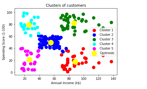
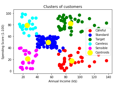
From the above output image, some following conclusions are made:
- Cluster 1: Clients in cluster 1 have high income and low spending score, which means that the clients in this cluster earns a very high income but don’t spend enough money. So, the clients can be named as Careful.
- Cluster 2: Clients in this cluster have an average salary and average spending score. So, these clusters of clients are Standard.
- Cluster 3: It consists of clients with high income and high spending scores, which means this cluster is supposed to be the main potential of mall marketing to understand what sort of products are being purchased by the clients. So, we can name it as Target.
- Cluster 4: The next cluster is of low income but high spending score clients, and so they can be called as Careless.
- Cluster 5: The last cluster is of clients with low income and low spending score, which means that they are the Sensible ones.
We can change the cluster label accordingly in the same code as per the observations for our clarity, and this is the following output that we get after changing the labels;
It can be clearly seen that our code is very well structured, simple, and does the job as per one's requirement. So, it is suggested that you can use the same code with any other business problem with a distinct dataset. You will only need to change to the indexes. Also, the complete code is not meant for dimensions greater than 2, as it will obstruct the execution of the last step i.e., the visualization phase. So, in that case, if you would be needed to reduce the dimension of the dataset to 2-D to execute the last section of code and plot the clusters.
Advantages of K-means clustering
- Easy to implement, robust, and understandable.
- Faster than hierarchical clustering, with large no. of variables.
- Forms tighter cluster.
- With diverse datasets, results are much better.
Disadvantages of K-means clustering
- Hard to find the value of k.
- Ordering of data strongly affects the output.
- Sensitive to rescaling.
- It does not perform clustering well if the geometry shape is complex.
Applications of K-means clustering
- To get an instinct about the composition of data that we are dealing with.
- Cluster-then-predicts: Distinct clusters are formed for different subgroups.
- It is effectively integrated into market segmentation, astronomy, computer vision, image segmentation, image compression, and analyzing the latest trends on the dynamic data.