Reinforcement Learning in AI

Reinforcement Learning in AI

1. Reinforcement Learning
   • Markov’s Decision Process
   • Q leaning
   • Greedy Decision Making
   • NIM Game
   • NIM Game Implementation with Python

Reinforcement Learning

Reinforcement Learning is about learning from experience, where agents are given a set of rewards when it performs well and gives accurate result or punishment when it performs poorly. This reward is given in the form of numerical values. And, agents here can be a physical robot or a virtual code that does some task. So, based on the feedback, the agent learns what actions it should take in the future.

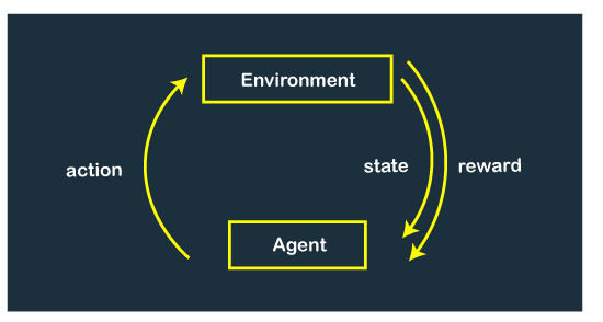
An agent is situated in an environment where all decisions are made, and feedback is given to the agent.

Suppose the environment puts the agent inside some state, and now the agent has to make some decision for that state. In return, based on the decision, an agent will get feedback from the environment, and feedback can be positive (reward) or negative (punishment). This way, the AI model can learn from the experience and figure out what things to do in the future and what not to do. In the reinforcement learning model, AI model can become intelligent not only with data but also with experience.

This technique can be used in various robots, like walking robots. For example, after a robot environment took each step, it returns a positive number as a reward, and each fall returns a negative number as a punishment.

This technique can also be used to train the virtual AI model. Suppose while predicting something, for every correct prediction, agent gets a positive number as a reward, and for every wrong prediction, it gets a negative number as a reward.

We need to formalize this idea of 'Agent', 'Environment', and 'Reward', which can be done using the Markov Decision Process.

Markov Decision Processes

Markov's Decision Process is the model for making a decision and representing actions, states, and rewards/punishments.

Suppose we have some states as shown in the figure below, and here one state leads to another state according to some probability distribution.

But, in this model, no agent had control over the whole process.

Now we have an agent, and it has the ability to choose the different actions. Suppose we have three different actions, each leading to a different path and further every state leading to more branching states, as shown in the figure below.

So, now from one state, each agent has different choices of actions leading to different states, and those states have further different probability distributions of going to different states.

Now, after every state, we can add some feedback, represented as 'r'. If r is positive, then it is some positive reward, and if r is negative, then it is punishment.

This is Markov’s Decision Model.

It has the following properties.

• Set of states S
• Set of actions Actions(S)
• Transition model P(s’ | s, a) – It means given a state ‘s’ if we take action ‘a’ then what are the probabilities that we will end up in next state ‘s`’.
• Reward function R(s, a, s’) – It means given s state ‘s’ if we take action ‘a’ and then end up in the next state ‘s`’ then what will the reward.

Let's consider an example of a simulated world where the agent has to navigate its way to destiny.

In the above picture, agent is the yellow dot similar to the robot, which will try to navigate its way to the green box, which is the destination, and once it reaches the destination, it gets some sort of reward.

Now, suppose our agent doesn't know the most accurate path to the destination, and some steps will return positive feedback, i.e., reward, and some will return the negative reward, i.e., punishment. In the picture below, suppose red blocks will return the negative feedback, and the agent doesn't know that yet.

Now agent will try a different path to reach the destination. Suppose agent initially not knowing takes action randomly and moves right and this action gives it negative feedback and agent will learn that going right should be avoided when in a state of the bottom left. This way, the agent will explore the space, learn and red mark the directions where it shouldn't go and from where it got negative feedback.

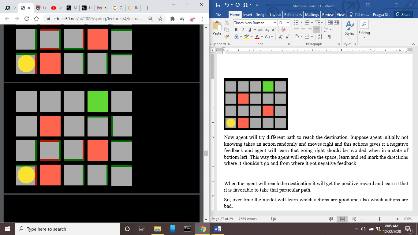
In the above figure, we can see that some entrances are marked by red and green. The red one signifies that the model has learned and they will not choose this path, and green lines show that the model has learned that they are safe paths. When the agent reaches the destination, it will get a positive reward and learn that it is favorable to take that particular path.

So, over time the model will learn which actions are good and also which actions are bad.

Q learning

Q learning is all about learning a function Q(s, a), which takes input some state 's' and some action 'a'. This Q function will estimate the value of reward after taking action 'a' in a state 's'.

Initially, we do not know what the value of the Q function is, but over time based on some experience, we can have the proper value of Q.

So, we can start by keeping the value 0 for all ‘s’ and ‘a’.

Q(s, a) =0 for all s,a

Then, the estimated value of Q(s, a) will be continuously updated based on experiences of rewards and punishments.

So, when we take action and receive a reward, we estimate the new value of Q(s, a) based on the current reward as well as expected future reward.

Then, we need to update the Q(s, a), taking into account the old as well as the new estimate.

This approach gives us an Algorithm that follows the following steps:

• Start with Q(s, a) = 0 for all s, a
• For every action ‘a’ in a state s and every time we observe a reward r.

Q(s, a) is updated by the following formula.

      Q(s, a) ? Q(s, a) + ?(new value estimate - Q(s, a))

Suppose our present value is 10, and the new value estimate is 20, then the difference is '10', so in this case, the estimate jumped by the value 10. And the value by which the present estimate value is changed or says how much we want to adjust the present and future estimate depend on '?’ alpha is also called the learning rate. Alpha also defines how much we value new information and how much we value old information. If alpha value is 1, then it means that we value new information as it simply overwrites the old estimate. And if alpha is 0, then old information is really valuable.

The new value estimate will be composed of two parts first is the reward ‘r’ if the action taken is 'a', and the second is the future reward estimate.

Q(s, a) ? Q(s, a) + ?((r + future reward estimate) - Q(s, a))

Now to figure out the future estimate value, we can take the maximum of all the possible actions we could take in the future.

Q(s, a) ? Q(s, a) + ?((r +max Q(s`, a`) - Q(s, a))

So, our Q learning function will be updated according to the above formula. So this function is updated not only on the basis of the reward but also by the expected future estimate value of Q in some state s` when the action taken is a`.

So, the main approach of this algorithm is that every time we get some new reward, we take that into account and update the value use it for future decisions. And there comes the idea of an algorithm called Greedy Decision-Making.

Greedy Decision-Making 

A Greedy Decision-Making Algorithm is implemented when we have a good estimate for every state and action, i.e., if we are in a state 's' and we want to know which actions we should take, then we consider the value of Q(s, a) for all possible actions. We will pick the action in which the value of Q(s, a) is highest.

So, at any given state, we can greedily say that for all my actions, this particular action gives me the highest estimated value so that we will choose this action.

But, there is one disadvantage of this approach, which affects the solution in the situations like where we have to find the best path to the destination, and we already know some action which returns some reward.

And we want our agent to figure out the best possible way to the destination. But when the agent always takes action it knows is the best, and it gets to the point of saying a particular square which agent has not explored yet, then the agent does not know about that particular action as it has never tried it.

But on the other side agent knows and has knowledge of the other action, which always leads to the destination. So, an agent might learn that it should always take the path that it already knows and get a reward instead of trying the new path and figuring out the best path to the destination.

In reinforcement learning, there is a tension between exploration and exploitation.

Exploitation- It is about only using the knowledge agent/AI already has, without exploring the other possibilities. Suppose AI knows a path that leads to destination and return reward so, AI/Agent will use that action or say the path to move forward.

Exploration- It is about exploring all the possible actions before taking the final decision. As suppose agent already have a knowledge of a particular path which leads to destination and returns the reward, then also the agent will explore the other path because there might be other path or says actions which can lead to the destination faster and return more rewards.

The agent who only exploits the information might be able to get the reward but mostly fail to find the best reward and cannot maximize its reward because it does not know the possibilities that are out there and which can only found by Exploring.

One approach to address this disadvantage is to use the epsilon-greedy algorithm.

In the epsilon-greedy Algorithm,

• We set ? equal to the number of random moves to explore through the choices of the actions and figure out and learn different possible actions.
• We choose the best move when the probability is 1- ?.
• We choose the random move when the probability is ?.

So, in the Greedy Algorithm, we always choose the best move, but in the epsilon greedy algorithm, sometimes we choose the best move and sometimes the random move.

This type of approach is one of the powerful approaches in Reinforcement learning because it allows you to choose the best possible move at the present moment. Still, sometimes it also allows you to explore and choose the random moves and various possible states and actions. After exploring various moves after we are confident that we have explored enough possibilities, then we can decrease the value of epsilon.

One of the most common applications of Reinforcement Learning is Game Playing.

Suppose we want to teach our AI agent to learn how to play the game, then first we have let our agent play the game and explore all the possibilities, and after the game is over, feedback reward is presented to the agent. Suppose AI agent has won the game it gets ‘1’ or ‘-1’otherwise. Then AI agent begins to learn and understand which actions are good and which are not.

NIM Game

Let’s consider the example of one game called NIM.

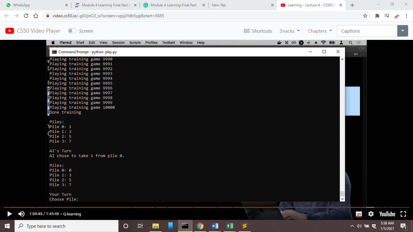
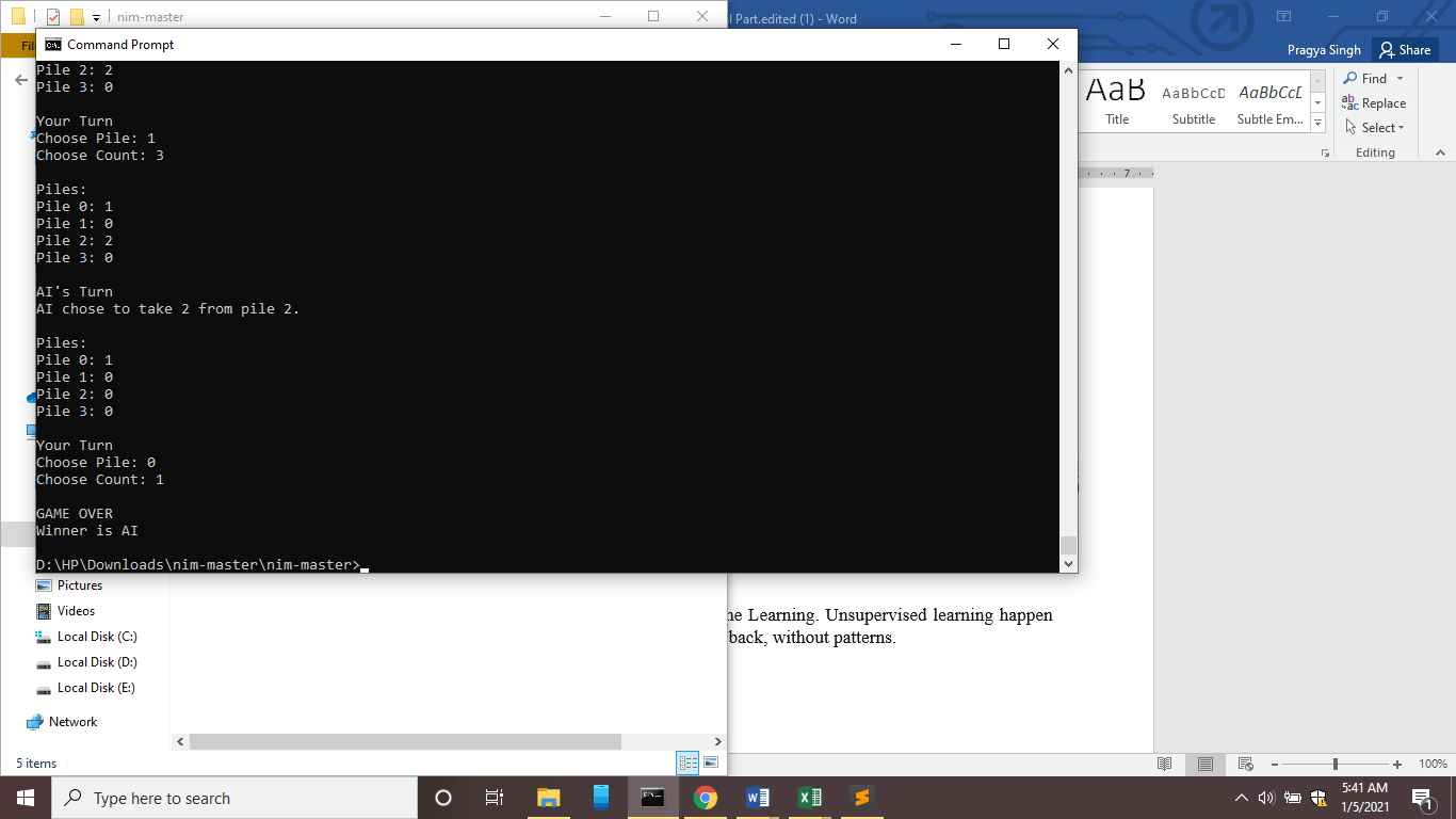
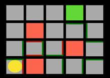
NIM is a game where multiple objects are piled in a certain way. And in the above picture, one object is piled in row1, three objects in row 2, five objects in row 3 and seven objects in row 4.

This basically is a two-player game, and each player has to remove any number of objects from a particular pile here, piles are represented as rows and the last person to remove the object will lose.

We can train an AI to play this game smartly, but we will start to train our AI agent by taking an untrained agent first and letting it play randomly and at last agent will get the reward 1 if it will win and -1 if it will lose. Initially, it will be very easy to win against this AI, but after this agent has played over 10,000 games and learned from its experiences, then it will smart enough to play this game, and it will hard enough to win against this AI agent which has the experience of 10,000 games.

Let’s see the implementation of NIMO game using Q learning.

Python Code for NIMO

First Step: Importing all the necessary libraries.

 import math
 import random
 import time 

Second Step: Defined a class with a name Nim.

1. First the function with name __init__ is defined to initialize the environment of the game, and the main components of NIM game are:

‘piles' : It is the list of a number of elements left in each pile.

‘player’: To indicate the turn of the player by 0 or 1.

‘winner’ : To indicate the winner by ‘None’, 0,1.

• Second function is defined with a name ‘available actions’, this function takes the list of the piles as input and returns the actions available in that state. Action is represented by (i, j) where j represents the number of items and i represents the pile number.
• Next function is other_player; it returns the player.
• Next switch_player function is used to switch the current player to the other player.
• The function 'move' is used to make a move i.e. action for the current player. And action should be in the form of the tuple, i.e. (i, j).

Then, we have defined conditions to check the errors, to invalidate any wrong input.

Then, we have updated the pile and defined the condition to check the error.

 class Nim():
     def __init__(self, initial=[1, 3, 5, 7]):
         self.piles = initial.copy()
         self.player = 0
         self.winner = None
     @classmethod
     def available_actions(cls, piles):
         actions = set()
         for i, pile in enumerate(piles):
             for j in range(1, pile + 1):
                 actions.add((i, j))
         return actions
     @classmethod
     def other_player(cls, player):
         return 0 if player == 1 else 1
     def switch_player(self):
         self.player = Nim.other_player(self.player)
     def move(self, action):
         pile, count = action
         # Check for errors
         if self.winner is not None:
             raise Exception("Game already won")
         elif pile < 0 or pile >= len(self.piles):
             raise Exception("Invalid pile")
         elif count < 1 or count > self.piles[pile]:
             raise Exception("Invalid number of objects")
 # Update pile
         self.piles[pile] -= count
         self.switch_player()
         # Check for a winner
         if all(pile == 0 for pile in self.piles):
             self.winner = self.player 

Third Step: We will define the class called NimAI in which we will define other player which will be AI agent using Q learning approach.

1. First, we have defined the function called __init__  in which we will initialize AI agent with an empty Q learning dictionary with some alpha rate and an epsilon rate.

The Q learning dictionary will map (state, action) to Q-value where state is the tuple of the number of piles left, and action is the tuple (i, j).

• Next, we have defined a function called ‘update’ which will update the Q learning model where an old state will be given and after some action is taken on that state it will be resulted in some new state and it will be updated and the reward received after taking that action.
• Next, function is get_q_value, and this function return the Q-value for the present state and action. And, it returns 0 if no Q-value exist in self.q.
• The next function is update_q_value, which will update the Q- value every time.

For the given previous Q-value ‘old_q’ and current reward ‘reward’ and an estimate of future rewards ‘future_reward’, the Q-value is updated for the state 'state' and the action 'action'.

Formula used is:

Q(s, a) <- old value estimate + alpha * (new value estimate - old value estimate)

Where,

old value estimate = Previous Q-value

alpha= learning rate new value estimate= It is the sum of current reward and the estimate future reward.

class NimAI():
     def __init__(self, alpha=0.5, epsilon=0.1):
         self.q = dict()
         self.alpha = alpha
         self.epsilon = epsilon
     def update(self, old_state, action, new_state, reward):
         old = self.get_q_value(old_state, action)
         best_future = self.best_future_reward(new_state)
         self.update_q_value(old_state, action, old, reward, best_future)
     def get_q_value(self, state, action):
         if (tuple(state), action) not in self.q:
             return 0
         else:
             q_value = self.q[(tuple(state), action)]
             return q_value
     def update_q_value(self, state, action, old_q, reward, future_rewards):
         update_q_value = old_q + self.alpha * (reward + future_rewards - old_q)
         self.q[(tuple(state), action)] =  update_q_value 

• The next function is best_future_reward with the parameters self and state.

For the given state, 'state' after considering all the possible states and action pairs (states, pair) available in that particular state and returns the action with the maximum Q-value.

We have considered Q-value as zero, when state action pair has no Q-value in self.q , And if there are no actions available in a state 'state' then it will return 0.

• The next function is choose_action, which returns the best action available for that state.

If the epsilon is False, then it will return the best action available in that state with the highest Q-value, and considering the Q-value 0 for the pairs that have no Q-values.

If the epsilon is True, it will choose the random available action based on the probability ‘self.epsilon’.

If multiple actions have the same Q-value, then any of those actions can be selected.

• Now, we can train our AI agent by playing n games against itself.

Following are the steps:

• Keep track of the last move made by either player.
• Make the game loop, and in that,
  • Keep track of the current state and action.
  • Keep track of the last state and action.
  • Make move
  • After the game is over, update the Q values with rewards.
  • If the game is continuing then, no rewards yet.
  • Return the trained AI

       def best_future_reward(self, state):
         actions = Nim.available_actions(state)
         if len(actions) == 0:
             return 0  
         best_value = 0
         for action in actions:
             q_value = self.get_q_value(state, action)
             if q_value > best_value:
                 best_value = q_value
             else:
                 continue
         return best_value
     def choose_action(self, state, epsilon=True):
         actions = list(Nim.available_actions(state))
         best_move = 0
         max_score = 0       
         random_action = random.choice(actions)
         for action in actions:
             if (tuple(state), action) in self.q:
                 q_value = self.get_q_value(state, action)
                 if  q_value > max_score:
                     best_move = action
                     max_score = q_value
             else:
                 q_value = 0 
         if best_move == None:
             best_move = random_action
         if epsilon == False:
             return best_move
         else:
             random_move = random.choices([best_move, random_action], weights=[self.epsilon, 1 - self.epsilon])[0]
             return random_move   
 def train(n):
     player = NimAI()
     # Play n games
     for i in range(n):
         print(f"Playing training game {i + 1}")
         game = Nim()
         # Keep track of last move made by either player
         last = {
             0: {"state": None, "action": None},
             1: {"state": None, "action": None}
         }
         # Game loop
         while True:
             # Keep track of current state and action
             state = game.piles.copy()
             action = player.choose_action(game.piles)
             # Keep track of last state and action
             last[game.player]["state"] = state
             last[game.player]["action"] = action
             # Make move
             game.move(action)
             new_state = game.piles.copy()
             # When game is over, update Q values with rewards
             if game.winner is not None:
                 player.update(state, action, new_state, -1)
                 player.update(
                     last[game.player]["state"],
                     last[game.player]["action"],
                     new_state,
                     1
                 )
                 break
             # If game is continuing, no rewards yet
             elif last[game.player]["state"] is not None:
                 player.update(
                     last[game.player]["state"],
                     last[game.player]["action"],
                     new_state,
                     0
                 )
     print("Done training")
     # Return the trained AI
     return player 

And then, below is the code for game between AI and human player.

 def play(ai, human_player=None):
     # If no player order set, choose human's order randomly
     if human_player is None:
         human_player = random.randint(0, 1)
     # Create new game
     game = Nim()
     # Game loop
     while True:
         # Print contents of piles
         print()
         print("Piles:")
         for i, pile in enumerate(game.piles):
             print(f"Pile {i}: {pile}")
         print()
         # Compute available actions
         available_actions = Nim.available_actions(game.piles)
         time.sleep(1)
         # Let human make a move
         if game.player == human_player:
             print("Your Turn")
             while True:
                 pile = int(input("Choose Pile: "))
                 count = int(input("Choose Count: "))
                 if (pile, count) in available_actions:
                     break
                 print("Invalid move, try again.")
         # Have AI make a move
         else:
             print("AI's Turn")
             pile, count = ai.choose_action(game.piles, epsilon=False)
             print(f"AI chose to take {count} from pile {pile}.")
         # Make move
         game.move((pile, count))
         # Check for winner
         if game.winner is not None:
             print()
             print("GAME OVER")
             winner = "Human" if game.winner == human_player else "AI"
             print(f"Winner is {winner}")
             return 

Above whole code is “nim.py”

Code for play.py is:

 from nim import train, play
  
 ai = train(10000)
 play(ai) 

Here we have trained our AI agent on 10,000 games.

Steps to run this code:

1. Save the above code in one file with .py extension.
2. Run this python file in command prompt
   • cd <directory location> “ENTER”
   • python nim.py “ENTER”
   • python play.py “ENTER”
   • AI agent will be trained and you can play the game.