Uninformed Search Strategies - Artificial Intelligence

Breadth-first search (BFS)

It is a simple search strategy where the root node is expanded first, then covering all other successors of the root node, further move to expand the next level nodes and the search continues until the goal node is not found.

BFS expands the shallowest (i.e., not deep) node first using FIFO (First in first out) order. Thus, new nodes (i.e., children of a parent node) remain in the queue and old unexpanded node which are shallower than the new nodes, get expanded first.

In BFS, goal test (a test to check whether the current state is a goal state or not) is applied to each node at the time of its generation rather when it is selected for expansion.

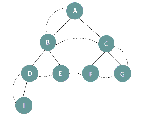
In the above figure, it is seen that the nodes are expanded level by level starting from the root node A till the last node I in the tree. Therefore, the BFS sequence followed is: A->B->C->D->E->F->G->I.

BFS Algorithm

• Set a variable NODE to the initial state, i.e., the root node.
• Set a variable GOAL which contains the value of the goal state.
• Loop each node by traversing level by level until the goal state is not found.
• While performing the looping, start removing the elements from the queue in FIFO order.
• If the goal state is found, return goal state otherwise continue the search.

The performance measure of BFS is as follows:

• Completeness: It is a complete strategy as it definitely finds the goal state.
• Optimality: It gives an optimal solution if the cost of each node is same.
• Space Complexity: The space complexity of BFS is O(b^d), i.e., it requires a huge amount of memory. Here, b is the branching factor and d denotes the depth/level of the tree
• Time Complexity: BFS consumes much time to reach the goal node for large instances.

Disadvantages of BFS

• The biggest disadvantage of BFS is that it requires a lot of memory space, therefore it is a memory bounded strategy.
• BFS is time taking search strategy because it expands the nodes breadthwise.

Note: BFS expands the nodes level by level, i.e., breadthwise, therefore it is also known as a Level search technique.

Uniform-cost search

Unlike BFS, this uninformed search explores nodes based on their path cost from the root node. It expands a node n having the lowest path cost g(n), where g(n) is the total cost from a root node to node n. Uniform-cost search is significantly different from the breadth-first search because of the following two reasons:

• First, the goal test is applied to a node only when it is selected for expansion not when it is first generated because the first goal node which is generated may be on a suboptimal path.
• Secondly, a goal test is added to a node, only when a better/ optimal path is found.

Thus, uniform-cost search expands nodes in a sequence of their optimal path cost because before exploring any node, it searches the optimal path. Also, the step cost is positive so, paths never get shorter when a new node is added in the search.

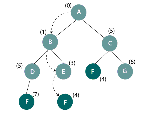
Uniform-cost search on a binary tree

In the above figure, it is seen that the goal-state is F and start/ initial state is A. There are three paths available to reach the goal node. We need to select an optimal path which may give the lowest total cost g(n). Therefore, A->B->E->F gives the optimal path cost i.e., 0+1+3+4=8.

Uniform-cost search Algorithm

• Set a variable NODE to the initial state, i.e., the root node and expand it.
• After expanding the root node, select one node having the lowest path cost and expand it further. Remember, the selection of the node should give an optimal path cost.
• If the goal node is searched with optimal value, return goal state, else carry on the search.

The performance measure of Uniform-cost search

• Completeness: It guarantees to reach the goal state.
• Optimality:  It gives optimal path cost solution for the search.
• Space and time complexity: The worst space and time complexity of the uniform-cost search is O(b^1+LC*/?^?).

Note: When the path cost is same for all the nodes, it behaves similar to BFS.

Disadvantages of Uniform-cost search

• It does not care about the number of steps a path has taken to reach the goal state.
• It may stick to an infinite loop if there is a path with infinite zero cost sequence.
• It works hard as it examines each node in search of lowest cost path.

Depth-first search

This search strategy explores the deepest node first, then backtracks to explore other nodes. It uses LIFO (Last in First Out) order, which is based on the stack, in order to expand the unexpanded nodes in the search tree. The search proceeds to the deepest level of the tree where it has no successors. This search expands nodes till infinity, i.e.,  the depth of the tree.

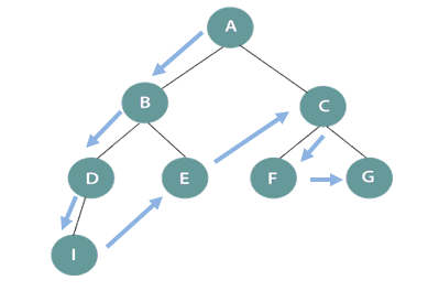
DFS search tree

In the above figure, DFS works starting from the initial node A (root node) and traversing in one direction deeply till node I and then backtrack to B and so on. Therefore,  the sequence will be A->B->D->I->E->C->F->G.

DFS Algorithm

• Set a variable NODE to the initial state, i.e., the root node.
• Set a variable GOAL which contains the value of the goal state.
• Loop each node by traversing deeply in one direction/path in search of the goal node.
• While performing the looping, start removing the elements from the stack in LIFO order.
• If the goal state is found, return goal state otherwise backtrack to expand nodes in other direction.

The performance measure of DFS

• Completeness: DFS does not guarantee to reach the goal state.
• Optimality: It does not give an optimal solution as it expands nodes in one direction deeply.
• Space complexity: It needs to store only a single path from the root node to the leaf node. Therefore, DFS has O(bm) space complexity where b is the branching factor(i.e., total no. of child nodes, a parent node have) and m is the maximum length of any path.
• Time complexity: DFS has O(b^m) time complexity.

Disadvantages of DFS

• It may get trapped in an infinite loop.
• It is also possible that it may not reach the goal state.
• DFS does not give an optimal solution.

Note: DFS uses the concept of backtracking to explore each node in a search tree.

Depth-limited search

This search strategy is similar to DFS with a little difference. The difference is that in depth-limited search, we limit the search by imposing a depth limit l to the depth of the search tree. It does not need to explore till infinity. As a result, the depth-first search is a special case of depth-limited search. when the limit l is infinite.

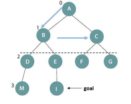
Depth-limited search on a binary tree

In the above figure, the depth-limit is 1. So, only level 0 and 1 get expanded in A->B->C DFS sequence, starting from the root node A till node B. It is not giving satisfactory result because we could not reach the goal node I.

Depth-limited search Algorithm

• Set a variable NODE to the initial state, i.e., the root node.
• Set a variable GOAL which contains the value of the goal state.
• Set a variable LIMIT which carries a depth-limit value.
• Loop each node by traversing in DFS manner till the depth-limit value.
• While performing the looping, start removing the elements from the stack in LIFO order.
• If the goal state is found, return goal state. Else terminate the search.

The performance measure of Depth-limited search          

• Completeness: Depth-limited search does not guarantee to reach the goal node.
• Optimality: It does not give an optimal solution as it expands the nodes till the depth-limit.
• Space Complexity: The space complexity of the depth-limited search is O(bl).
• Time Complexity: The time complexity of the depth-limited search is O(b^l).

Disadvantages of Depth-limited search

• This search strategy is not complete.
• It does not provide an optimal solution.

Note: Depth-limit search terminates with two kinds of failures: the standard failure value indicates “no solution," and cut-off value, which indicates “no solution within the depth-limit."

Iterative deepening depth-first search/ Iterative deepening search

This search is a combination of BFS and DFS, as BFS guarantees to reach the goal node and DFS occupies less memory space. Therefore, iterative deepening search combines these two advantages of BFS and DFS to reach the goal node. It gradually increases the depth-limit from 0,1,2 and so on and reach the goal node.

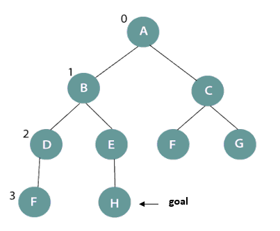
In the above figure, the goal node is H and initial depth-limit =[0-1]. So, it will expand level 0 and 1 and will terminate with A->B->C sequence. Further, change the depth-limit =[0-3], it will again expand the nodes from level 0 till level 3 and the search terminate with A->B->D->F->E->H sequence where H is the desired goal node.

Iterative deepening search Algorithm

• Explore the nodes in DFS order.
• Set a LIMIT variable with a limit value.
• Loop each node up to the limit value and further increase the limit value accordingly.
• Terminate the search when the goal state is found.

The performance measure of Iterative deepening search

• Completeness: Iterative deepening search may or may not reach the goal state.
• Optimality: It does not give an optimal solution always.
• Space Complexity: It has the same space complexity as BFS, i.e., O(b^d).
• Time Complexity: It has O(d) time complexity.

Disadvantages of Iterative deepening search

• The drawback of iterative deepening search is that it seems wasteful because it generates states multiple times.

Note: Generally, iterative deepening search is required when the search space is large, and the depth of the solution is unknown.

Bidirectional search

The strategy behind the bidirectional search is to run two searches simultaneously--one forward search from the initial state and other from the backside of the goal--hoping that both searches will meet in the middle. As soon as the two searches intersect one another, the bidirectional search terminates with the goal node. This search is implemented by replacing the goal test to check if the two searches intersect. Because if they do so, it means a solution is found.

The performance measure of Bidirectional search

• Complete: Bidirectional search is complete.
• Optimal: It gives an optimal solution.
• Time and space complexity: Bidirectional search has O(b^d/2)

Disadvantage of Bidirectional Search

• It requires a lot of memory space.

Related Posts:

• Constraint Satisfaction Problems in Artificial Intelligence
• Alpha-beta Pruning | Artificial Intelligence
• Adversarial Search in Artificial Intelligence
• Heuristic Functions in Artificial Intelligence
• Local Search Algorithms and Optimization Problem
• Informed Search/Heuristic Search
• Problem-solving in Artificial Intelligence
• Artificial Intelligence Tutorial | AI Tutorial
• Hill Climbing Algorithm
• Theory of First-order Logic
• Inference Rules in Proposition Logic