Matlab Algebra
Up until now, we have seen that every one of the models work in MATLAB just as its GNU, then again called Octave. In any case, for addressing fundamental mathematical conditions, both MATLAB and Octave are minimal unique, so we will attempt to cover in MATLAB and alternative Octave in independent areas.
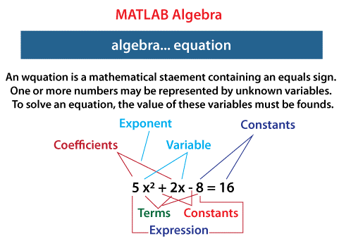
Variable based math that is ALGEBRA is all about the investigation of numerical images and rules for controlling these symbol images. Here factors variables are utilized to store/address amounts. There are sure in-assembled strategies in Matlab to address polynomial math conditions. Underlying foundations of conditions, tackling for x, working on an articulation are a few things we can act in MATLAB.
Basic Algebraic Equations Solving in MATLAB
For solving and finding algebraic equations solutions, the solve function is used. In its easiest format, the function called solve(), takes arguments as the equation is in “ “ quotes.
Example, let us find solution for y in the equation y-6 = 0
solve('y-6=0')The above statement MATLAB will execute and return result as follows-
ans =
   6
You can also use above solve function as follows –
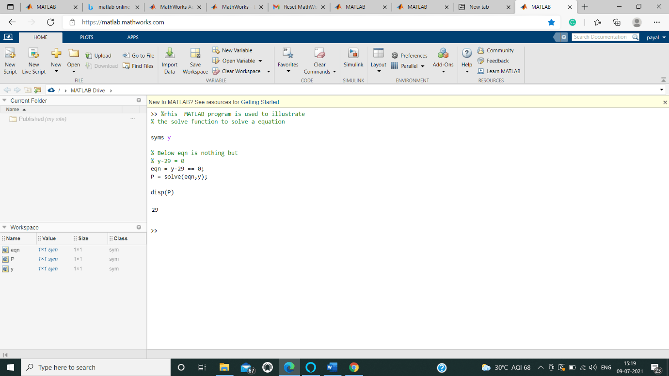
We Created a script file code to illustrate the above function-
%this  MATLAB program is used to illustrate
% the solve function to solve a equation


syms y


% Below eqn is nothing but
% y-29 = 0
eqn = y-29 == 0;
P = solve(eqn,y);


disp(P)
Output:
Factorization of an expression and Simplification:
To find factors of or simplify an expression we use factor() function and simplify() function respectively. When we use many symbolic functions in our code, we must declare that variables as symbolic.
Factor Syntax:
factor(any type of expression)
    or
factor(any_integer)
Simplify Syntax:
simplify(any type of expression)If an expression is passed into factor() function, then it returns an array of factors. If an integer is passed into factor() function, then it returns prime factorization of the given integer.
We Created a script file code to illustrate the above function-
% to find factors to illustrate
% factor function


syms p
syms q


% prime factorization of
% any given integer
factor(29)


% factors of
% expressions p^4-q^4
factor(p^4-q^4)
factor(p^6-1)
Output:
ans =


    29

ans =

[p - q, p + q, p^2 + q^2]


ans =

[p - 1, p + 1, p^2 + p + 1, p^2 - p + 1]
Solve linear system of linear equation
A linear system can be solved with help of both function mldivide and linsolve to think about execution.
mldivide is the prescribed method to address most direct frameworks of conditions in MATLAB ®. Be that as it may, the capacity plays out a few keeps an eye on the info lattice to decide if it has any exceptional properties. In the event that you think about the properties of the coefficient grid early, then, at that point you can utilize linsolve to stay away from tedious checks for enormous matrices.
Utility function helps in solving matrix equation easily
Mldivide “\”
To Solve linear equations systems like Px = Q for x
Syntax
x=P\Q
x= mldivide(P,Q)
Description
x = P\Q solves the given linear equations P*x = Q. The matrices P and Q must have the same rows. MATLAB® sends a message for warning if P is nearly singular, but gives the calculation regardless of any issue.
Example:
A1 = magic(4);
B1 = [14; 14; 14; 14];
x = A1\B1
Output:
A1 = magic(4);
B1 = [14; 14; 14;14];
x = A1\B1
Warning: Matrix is close to singular or badly scaled. Results may be inaccurate. RCOND =  4.625929e-18.
x =


    0.3725
    0.2941
    0.5294
    0.4510
Linsolve()
It is used to solve the linear system of equations.
Syntax
X= linsolve(P,Q)
X= limsolve(P,Q,opts)
[x,r] =linsolve(_________)
Description
X= linsolve(p,q) solves the linear system equation pX = q using any of these methods:
Example
A1 = tril(magic(1e4));
opts.LT = true;
b1 = ones(size(A1,2),1);
tic
x1 = A1\b1;
o1 = toc
tic
x2 = linsolve(A1,b1,opts);
o2 = toc
speedup = o1/o2
Output:
t1 =


    0.0825


t2 =


    0.0279
speedup = t1/t2


speedup =


    2.9545
Solving Quadratic Equations in MATLAB
To solve higher order equations, we use the solve() function. Roots of the equation is returned in the form of an array.
To solves the quadratic equation x2 -8x +16 = 0.
We Created a script file code to illustrate the above function-
eq1 = 'x^2 -8*x + 16 = 0';
s1 = solve(eq1);
disp('The first root of the quadratic equation x2 -8x +16 = 0.is: '), disp(s1(1));
disp('The second root of the quadratic equation x2 -8x +16 = 0. is: '), disp(s1(2));
After we run the above script file, we get the following expected result -
The first root of the quadratic equation x2 -8x +24 = 0.is: 4
The first root of the quadratic equation x2 -8x +24 = 0.is: 4
MATLAB Higher Order Equations solution
Roots are lengthy of higher order degree equations, and may contain many terms. Roots values can be obtained by converting to double datatype. The fourth order degree equation is solved x4 - 8x3 + 3x2 - 5x + 9 = 0.
We have Created a script file code -
eq = 'x^4 - 7*x^3 + 3*x^2 - 5*x + 9 = 0';
s = solve(eq);
disp('The first root of the quadratic equation x4 - 8x3 + 3x2 - 5x + 9 = 0 is'), disp(s(1));
disp(' The second root of the quadratic equation x4 - 8x3 + 3x2 - 5x + 9 = 0 is'), disp(s(2));
disp(' The third root of the quadratic equation x4 - 8x3 + 3x2 - 5x + 9 = 0 .is''), disp(s(3));
disp(' The fourth root of the quadratic equation x4 – 8 x3 + 3x2 - 5x + 9 = 0 .is''), disp(s(4));


% converting equation roots to double data type
disp(' The first root  numeric value of the quadratic equation x4 - 8x3 + 3x2 - 5x + 9 = 0 .is''), disp(double(s(1)));
disp(' The second root numeric value of the quadratic equation x4 - 8x3 + 3x2 - 5x + 9 = 0 .is''), disp(double(s(2)));
disp(' The third root numeric value of the quadratic equation x4 - 8x3 + 3x2 - 5x + 9 = 0 .is''), disp(double(s(3)));
disp(' The fourth root numeric value of the quadratic equation x4 - 8x3 + 3x2 - 5x + 9 = 0 .is''), disp(double(s(4)));
After we run the above script file, we get the following expected result -
The first root of the quadratic equation x4 - 8x3 + 3x2 - 5x + 9 = 0 is 6.630396332390718431485053218985
The second root of the quadratic equation x4 - 8x3 + 3x2 - 5x + 9 = 0 is 1.0597804633025896291682772499885
The third root of the quadratic equation x4 - 8x3 + 3x2 - 5x + 9 = 0 is - 0.34508839784665403032666523448675 - 1.0778362954630176596831109269793*i
The fourth root of the quadratic equation x4 - 8x3 + 3x2 - 5x + 9 = 0 is - 0.34508839784665403032666523448675 + 1.0778362954630176596831109269793*i
The first root numeric value of the quadratic equation x4 - 8x3 + 3x2 - 5x + 9 = 0 is   6.6304
The second root numeric value of the quadratic equation x4 - 8x3 + 3x2 - 5x + 9 = 0 is   1.0598
The third root numeric value of the quadratic equation x4 - 8x3 + 3x2 - 5x + 9 = 0 is   -0.3451 - 1.0778i
The fouth root numeric value of the quadratic equation x4 - 8x3 + 3x2 - 5x + 9 = 0 is   -0.3451 + 1.0778i
MATLAB Equations - Expanding and Collecting
The expand() function and the collect() function expands exponentially and collects an equation variables respectively. The following instances demonstrates the function usage clearly.
When we will work with different symbolic functions, we must declare that the variables are symbolic in nature.
We Created a script file code to illustrate the above function-
syms p   %representing symbolic variable p
syms q   %representing symbolic variable p
% we are expanding equations
expand((p-6)*(p+9))
expand((p+2)*(p-3)*(p-5)*(p+7))
expand(sin(3*p))
expand(cos(p+q))

% collecting equations
collect(p^5 *(p-7))
collect(p^4*(p-3)*(p-5))
After we run the above script file, we get the following expected result -
ans =

p^2 + 3*p - 54


ans =

p^4 + p^3 - 43*p^2 + 23*p + 210


ans =

4*cos(p)^2*sin(p) - sin(p)


ans =

cos(p)*cos(q) - sin(p)*sin(q)


ans =

p^6 - 7*p^5


ans =

p^6 - 8*p^5 + 15 *p ^ 4


   x ^ 6 – 8 * x ^ 5 + 15* x ^ 4