In this section, we portray a greater amount of MATLAB's illustrations graphic functions and the most well-known methods of controlling and redoing graphics. Let’s type help designs, help graph2d (for two-dimensional designs orders), help graph3d (for three-dimensional graphics).

We will start this part by talking about more functions that ease out the task of representing dynamics of complex problems, just as a portion of the other most regularly utilized plotting orders. Then, at that point, we will examine techniques for modifying and controlling illustrations. At last, we will present a few special functions in Matlab for making and adjusting complex mathematical concepts with beautiful graphical illustrations.

MATLAB stem3()

Stem() technique in MATLAB is a kind of plotting strategy to address any sort of information in a discrete structure. This technique creates a plot as upward lines being stretched out from the bases line, having little circles at tips which addresses the specific worth of the given information. In contrast to the function plot() work, it doesn't join the qualities focuses with one another to make a nonstop chart, rather it accentuates the way that the information focuses are discrete, not persistent.

Syntax:

stem3(q)
stem3(q, w, e)
stem3(.,……….…..,'fill')
stem3(……….....,LineSpec)
i = stem3(...)

Example:

Creating a 3D plot of stem to visualize two variables function.

figure
X1 = 0 : pi / 300 : 3 * pi;


Y1 = exp (-7 * X1 / 6 ) .* cos(3 * X1 ) ;
stem (X1 , Y1)

Output:

Stem objects are viewed as one of a kind identifiers. These permit a client to alter properties for a stem various object at the pursue time it is being made. It upholds practically all normal properties from MATLAB that are upheld by a nonstop plotting capacity plot(). Notwithstanding those properties, it has its own novel properties that give a wide scope of augmentations to be applied to a discrete diagram produced from the stem() technique.

MATLAB Stairs()

To draw time history we use Stairstep plots for digitally perfect sampled-record models.

Syntax

stairs(r)
stairs(r,y)
stairs(........,LineSpec)

Example

We are Creating a stairs Plot

r^ 3=3sin6t,0= t1 =3p  
y1= r sin t1  
t1=linspace(0,3 * pi , 300 );  
r1=sqrt(abs(3 * sin(8*t)));  
y1 = r. * sin( t1 );  
stairs(t1 , y1);  
axis[0 pi 0 inf]);

Output:

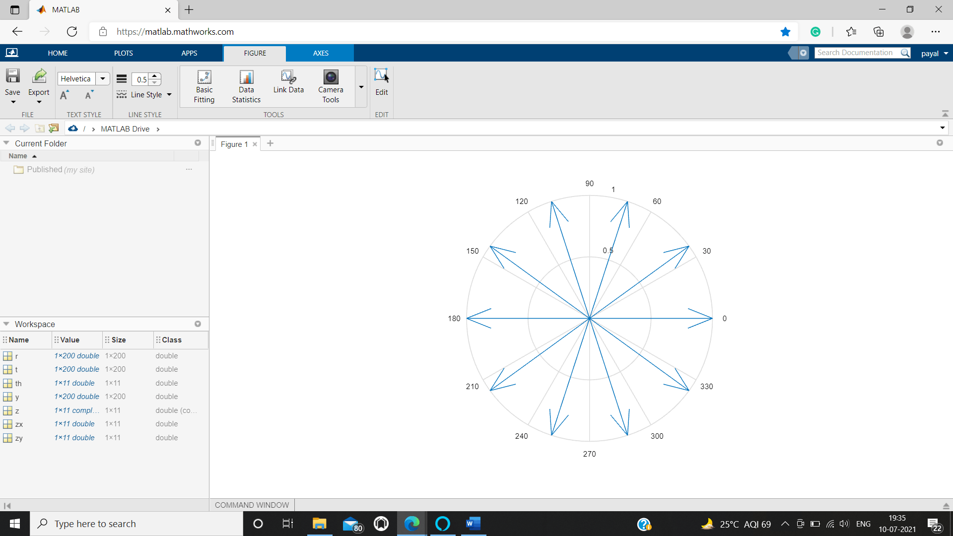
MATLAB compass()

To shows the vectors of velocity as arrows of the origin a compass plot is used. Cartesian coordinates X, Y, and Z are plotted on a circular grid as shown.

Syntax

compass(w,e)
compass(r)
compass(…....,LineSpec)
l = compass(….....)

Example

We are Creating a compass Plot.

o=cost+isint,-p=t=p  
th1=-pi : pi/6:pi;  
zx1=cos (th1);  
zy1=sin (th1);  
o=zx1+i*zy1;  
compass(o)

Output:

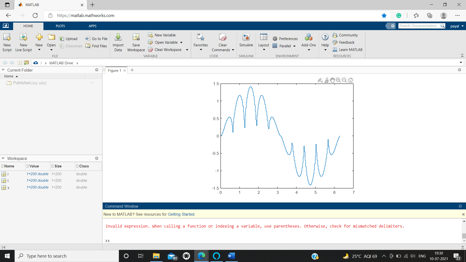
MATLAB Polar Plots()

Plots are the method of displaying the examples or pattern in a graphically manner which are straightforward and settle on the important business choices. They can be an incredible assistance to the ignorant crowd without or a little foundation information about the subject. There are various kinds of plots that are utilized to show various examples or patterns. For instance: If we need to view the appropriation of a particular element in a specific region then we can utilize the dissipate plot. Thus, you can pick the kind of plot contingent upon the business necessities.

Syntax:

 polar(&θ;, ra)

This creates angle θ polar plot of and radial distance of ra.

Example

We are Creating a Polar Plot

r1^3=3sin8t,0=t=3p  
t1=linspace(0, 3*pi,300);  
r1=sqrt(abs(3 * sin(8 * t1)))  
polar(t1, r1)

Output:

r =
  Columns 1 through 15
      0    0.5607    0.7881    0.9551    1.0866    1.1915    1.2742    1.3368    1.3806    1.4063    1.4142    1.4045    1.3770    1.3314    1.2669


  Columns 16 through 30
    1.1821    1.0747    0.9402    0.7687    0.5322    0.1777    0.5879    0.8068    0.9696    1.0982    1.2008    1.2813    1.3420    1.3839    1.4078


  Columns 31 through 45
    1.4140    1.4025    1.3733    1.3258    1.2593    1.1724    1.0626    0.9250    0.7488    0.5019    0.2513    0.6137    0.8251    0.9838    1.1095


  Columns 46 through 60
    1.2098    1.2883    1.3470    1.3871    1.4093    1.4137    1.4004    1.3694    1.3200    1.2516    1.1625    1.0502    0.9093    0.7282    0.4696
  Columns 61 through 75
    0.3077    0.6384    0.8428    0.9977    1.1206    1.2186    1.2950    1.3519    1.3902    1.4105    1.4131    1.3981    1.3653    1.3141    1.2436
  Columns 76 through 90
    1.1524    1.0375    0.8933    0.7070    0.4349    0.3553    0.6622    0.8601    1.0113    1.1315    1.2271    1.3016    1.3565    1.3930    1.4115
  Columns 91 through 105
    1.4124    1.3956    1.3610    1.3079    1.2355    1.1421    1.0246    0.8769    0.6850    0.3971    0.3971    0.6850    0.8769    1.0246    1.1421

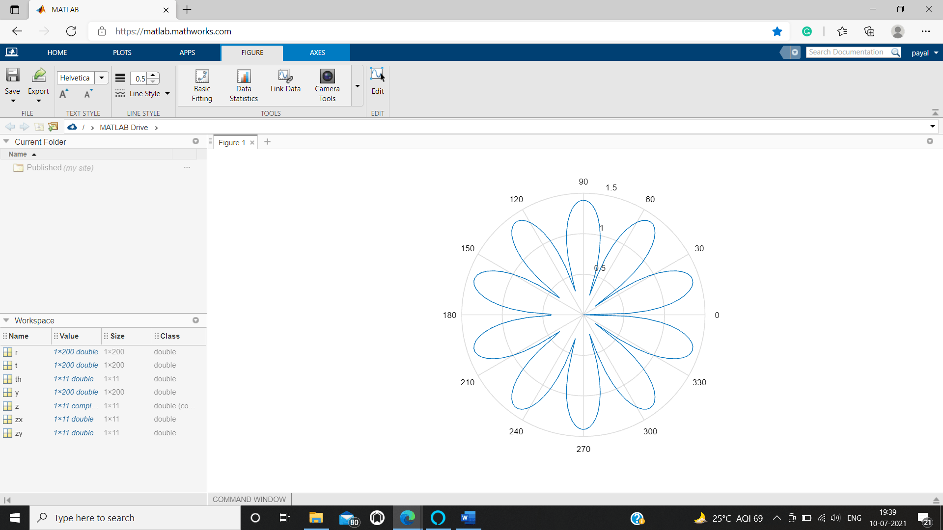
The polar plot is the sort of plot which is for the most part used to make various kinds of plots like line plot, disperse plot in their individual polar directions. They are likewise useful in changing the tomahawks in the polar plots. In Matlab, polar plots can be plotted by utilizing the capacity polarplot(). If it's not too much trouble, find the underneath linguistic uses which clarify the various properties of the polar plot.

There are various plots that can be plotted with the assistance of polar plots like histogram, line and disperse plot however in the above part, we have examined the customization of line plots utilizing the polar directions. Essentially, different plots can likewise be plotted and redone similarly.

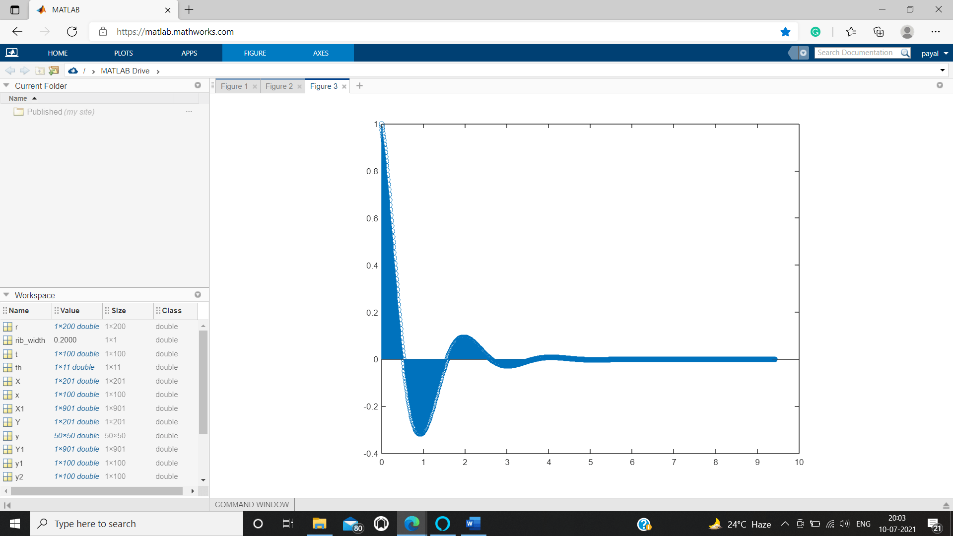
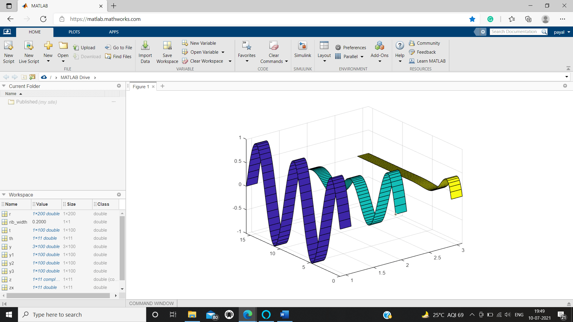
MATLAB ribbon()

It creates a ribbon plot.

Syntax

ribbon(h)
o = 2 : size(u,2).
ribbon(h,u)
ribbon(h,u,width)
ribbon(axes_handle,…………..)
x= ribbon(…………...)

Example

We are Creating a 3D ribbon Plot.

u_1=sin?(l),u_2=e^(-.15l) sin?(l)  
u_3=e ^ (-.8l) sin?(l)  
for 0= l= 5p  
l=linspace (0, 5 * pi, 100);  
u1=sin(t);  
u2=exp(-.15*l). * sin(l);  
u3=exp(-.8 * l). * sin(l);  
u=[u1; u2; u3];  
rib_width=0.2;  
ribbon(l',u',rib_width)

Output:

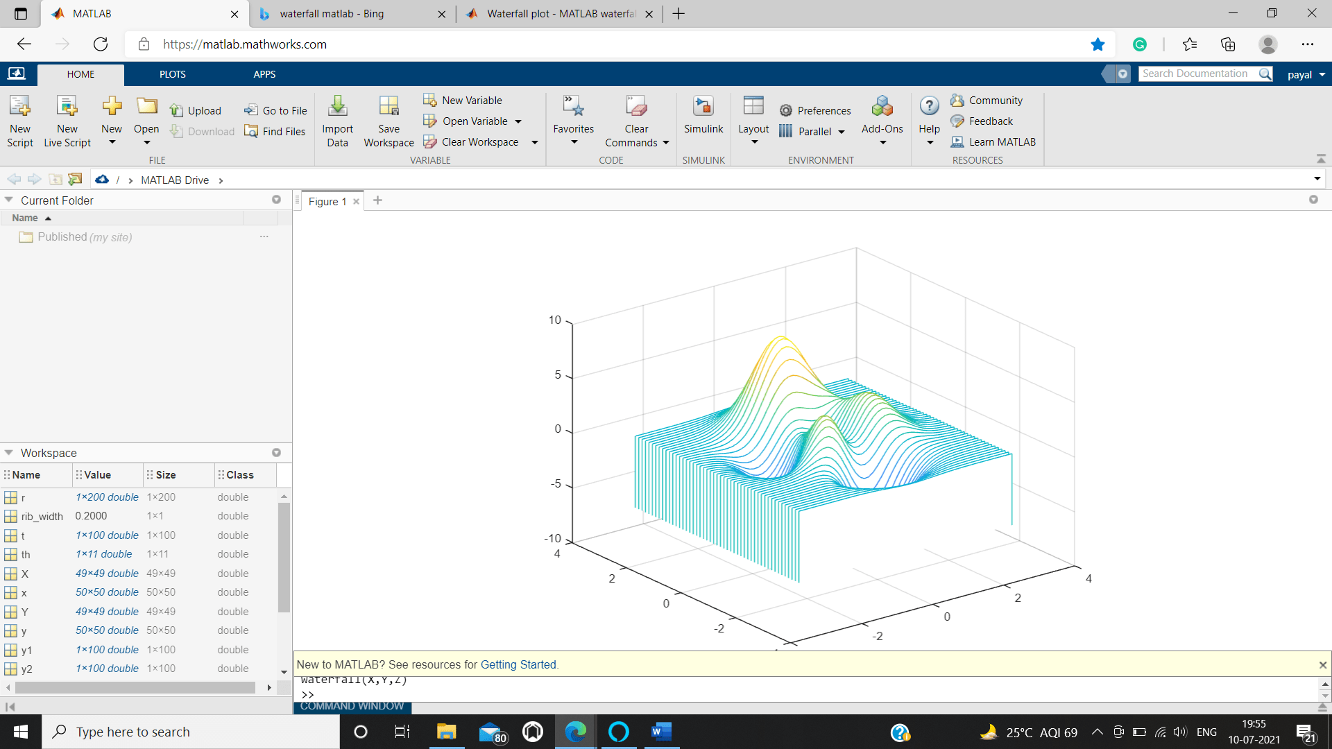
MATLAB waterfall()

To draws a mesh, the waterfall function is used, same as to the meshz function, but from the given columns of the matrices it does not create lines.

Syntax

waterfall(v)
waterfall(u,w,v)
waterfall(...,…y)
i = waterfall(.............)

Example

We are Creating a 3D waterfall Plot.

[w,e] = meshgrid(-4 :.129:3);
o = peaks(w , e);
waterfall(w ,e ,o)

Output:

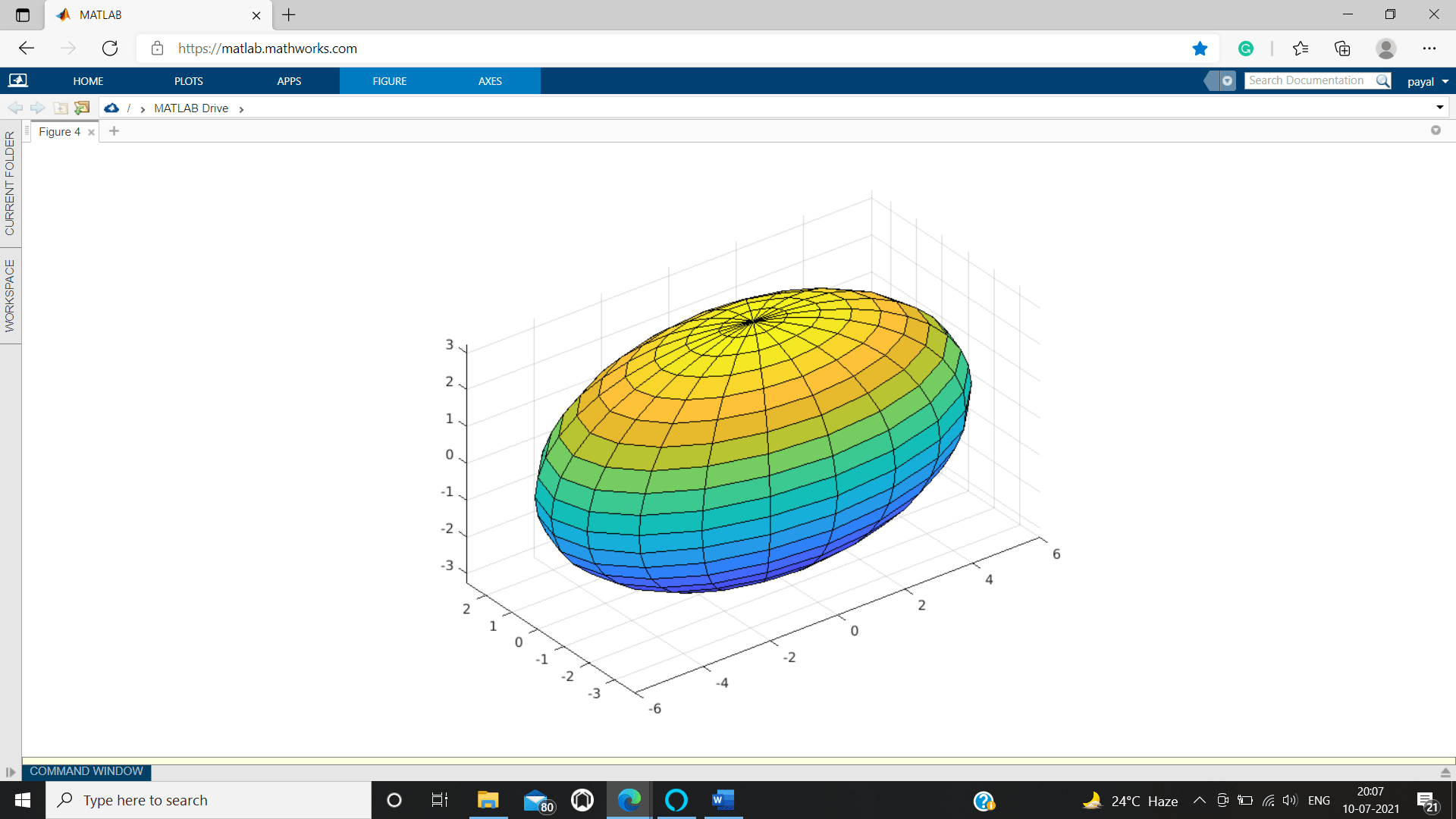
MATLAB ellipsoid()

It generates an ellipsoid function.

Syntax

[x,y,z] = ellipsoid(x,y,z,tx,ty,tz,n)
[x,y,z] = ellipsoid(x,y,z,xt,yt,z)
ellipsoid(………...)

Example

x=0;y=0;z=0;  
tx=1;ty=2;tz=0.6;  
ellipsoid(x,y,z,tx,ty,tz)  
axis('axis equal')

Output:

MATLAB cylinder()

Cylinder() function is an inbuilt 3D plotting capacity in MATLAB which is explicit to produce the barrel shaped items. This can be utilized to get the qualities for x, y, and z-directions of a chamber without plotting the yield or can be utilized to view the chamber contingent upon the information boundaries given in the capacity call.

The drawing of the barrel shaped 3D plot article can be completed by the recovered x, y, and z-facilitates utilizing surf() or cross mess() work, In MATLAB programming.

Syntax

[q, w, e] = cylinder
[q, w, e] = cylinder(s)
[q, w, e] = cylinder(s,n)
cylinder(...........)

Example

q=sin?(4p z)+3  
0=t=1,0=?=4?  
t=[0: .03:1]';  
q=sin(4*pi*t)+3;  
cyclinder(q), axis square

Output:

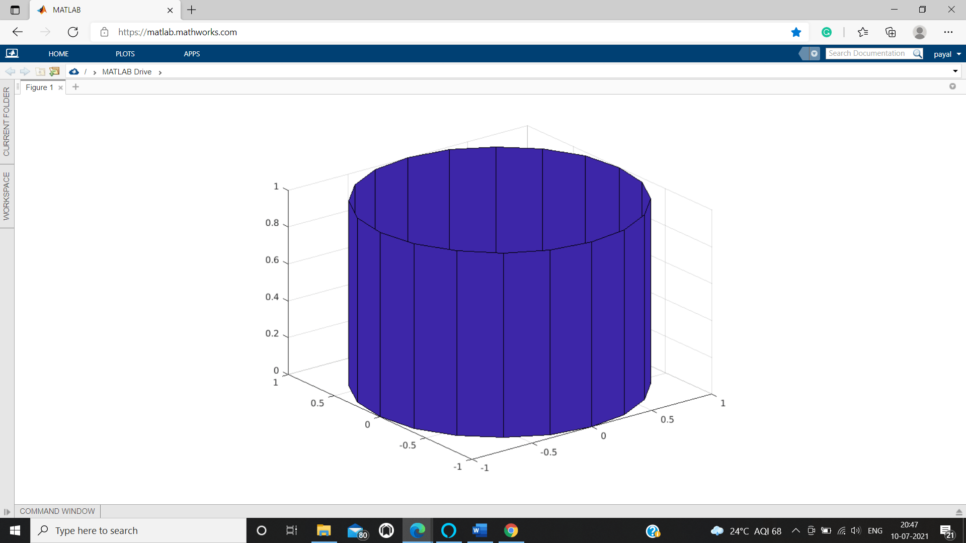
MATLAB broadens its component for the capacity chamber to make a chamber object with numerous range esteems for various countenances of it. It is feasible to accomplish by utilizing an articulation with depending variable as the unique information an incentive for the info boundary 'radius'.

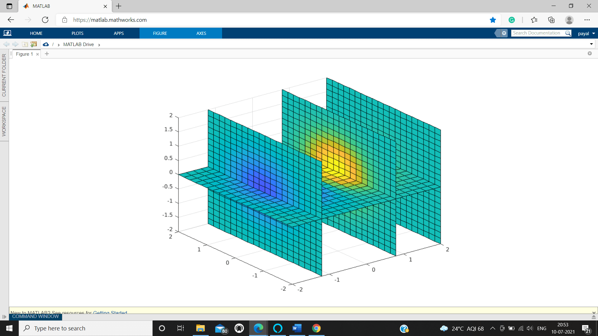
MATLAB slice()

To represent orthogonal slice planes we use 3D slice plots through volumetric huge data.

Syntax

slice(w,tx,ty,tz)
slice(X1,Y1,Z1,V,tx,ty,tz)
slice(V,Xo,Yo,Zo)
slice(X1,Y1,Z1,V,Xo,Yo,Zo)
slice(…..,'allmethod')
slice(axes_of_handle,...)
i = slice(………………....)

Example

[X2,Y2,Z2] = meshgrid(-3:.3:3);
V = X2.*exp(-X2.^3-Y2.^3-Z2.^3);


X1slice = [-1.3,0.9,3];   
Y1slice = [];
Z1slice = 0;
slice(X2,Y2,Z2,V,x1slice,y1slice,z1slice)

Output:

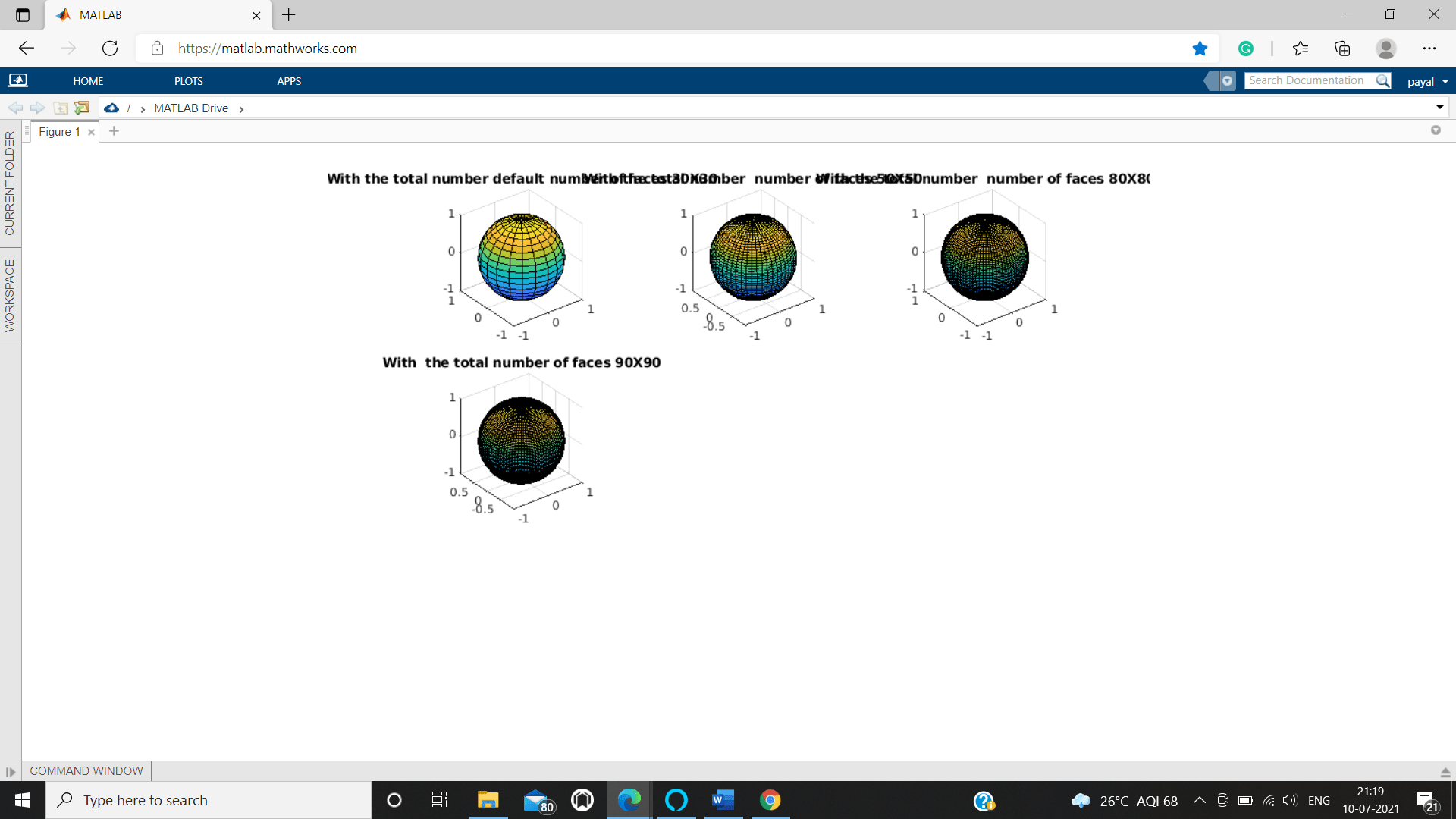
Matlab sphere function

MATLAB fuses the capacity sphere() which can be utilized to make a three-dimensional sphere. Since the capacity manages a three-dimensional chart, the yield from the capacity is gotten with three-axes co-ordinates.

Along these lines MATLAB writing computer programs is upheld by making three-dimensional circle plots utilizing the capacity circle. The capacity likewise gives adaptability to modify the presentation of the plots during the creation just as altering the showcase after the plot is made.

Example:

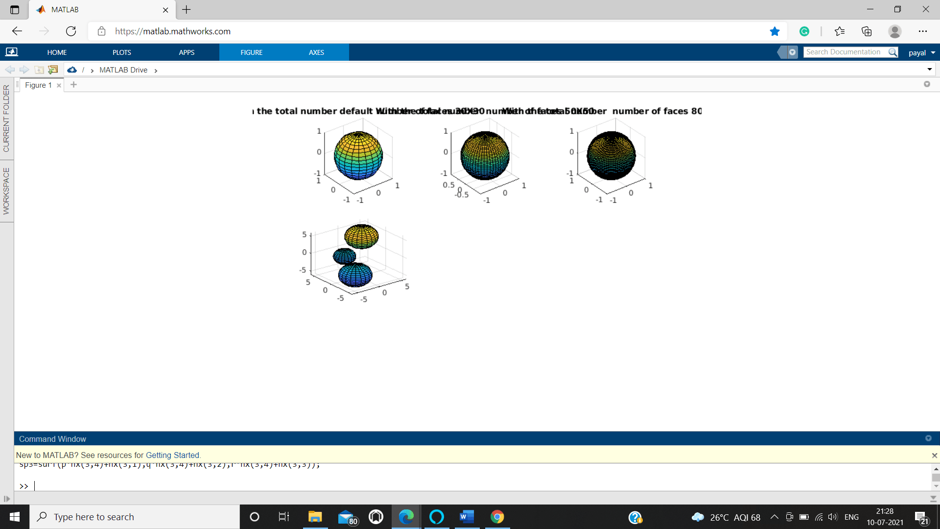
we are generating 4 different size of spheres viewing them in 4 segments of only single layouts.

Code:

tiledlayout(3,3);
pxy1 = nexttile;
sphere(pxy1);
axis equal
title('With the total number default number of faces 30X30')
pxy2 = nexttile;
sphere(pxy2,50)
axis equal
title('With the total number  number of faces 50X50')
pxy3 = nexttile;
sphere(pxy3,80)
axis equal
title('With the total number  number of faces 80X80')
pxy4 = nexttile;
sphere(pxy4,90)
axis equal
title('With  the total number of faces 90X90

Output:

For Multiple Spheres Setting Radius from An input type Array or matrix

As we have examined before, the sphere function capacity can likewise be utilized to make numerous circles in a solitary design. The origin and the radius can be set distinctively for every one of those circles by pronouncing the sweep esteems as a cluster or matrix.

Example:

clc
clear %command to clear screen
[p2 q2 r2] = sphere;
nx2 =  [2 2, 3 3;-2 -3 -2 3;0 9 -2 2];
sp3 = surf(p*nx(1,4)+nx(1,1),q*nx(1 , 4)+ nx( 1, 2),r*nx(1,4)+nx(1,3));
hold on
sp2 = surf(p * nx2(2 , 4) + nx2(2 , 1) , q * nx2(2 , 4) + nx2(2 ,2) , r * nx2(2 , 4) +  nx2(2,3));
hold on
sp4 = surf( p *  nx2(3,4) + nx2(3 ,  1) , q * nx2 (3 , 4) + nx2(3 , 2) , r * nx2 (3 , 4) + nx2(3 , 3));

Output:

MATLAB Tutorial

MATLAB Tutorial

MATLAB special graphic function

MATLAB stem3()

MATLAB Stairs()

MATLAB compass()

MATLAB Polar Plots()

MATLAB ribbon()

MATLAB waterfall()

MATLAB ellipsoid()

MATLAB cylinder()

MATLAB slice()

Matlab sphere function