MATLAB Transform
MATLAB furnishes for working with changes, for example, the Laplace and Fourier changes. Changes are utilized in science and designing as an instrument for improving on investigation and take a gander at information from another point.
For instance, the Fourier change permits us to change over a sign addressed as an element of time to an element of recurrence. Laplace change permits us to change a differential condition over to an arithmetical condition.
To play with mathematical operations like Laplace, Fourier and Fast Fourier transforms, MATLAB offers commands to support these operations -> Laplace() function, Fast Fourier transforms function.
Laplace Transform (How it is used?)
Let us understand how this function works with the help of steps involved in our example.
Step1:
The Laplace transform of any function, suppose g( t1 ), a function of time is used in our example.
Step2:
Laplace transform is also represented in the form à transform of g(t) to G(s).
Step3:
We can watch this transformation process by converting f( t1), a function of any variable t1, into another function F(s1) , with another variable s1.
Step4:
Differential equations into algebraic is changed by using Laplace transform.
To calculate a Laplace transform of a function f(t).
laplace( g( t1 ) )Example:
We can now execute a script containing the Laplace transform example.
Run the following code:
syms s1 t1 a1 b1 w1


laplace(a1)
laplace(t1 ^ 3)
laplace(t1 ^ 9)
laplace(exp( -b1 * t1))
laplace(sin(w1 * t1))
laplace(cos(w1 * t1))
Output:
ans =

1 / s ^ 2


ans =

6 / s ^ 4


ans =

362880 / s ^ 10


ans =

1 / ( b1 + s)


ans =

t1 / (s ^ 2 + t1 ^ 2)


ans =

s / (s ^ 2 + t1 ^ 2)
Inverse of Laplace Transform
To compute the inverse Laplace transform in Matlab, we use the command ilaplace.
Example:
ilaplace(1 / e ^ 4)
ans =
   e ^ 4 / 4
Example to find inverse of laplace transform.
syms e f a b w


ilaplace( 1/ e ^ 8)
ilaplace(2 / (w + e ))
ilaplace(e / ( e ^ 2 + 4 ))
ilaplace(exp( - b * f ))
ilaplace(w / (e ^ 3 + w ^ 3 ))
ilaplace(e / (e ^ 3 + w ^ 3 ))
Output:
ans =

t ^ 7 / 5040


ans =

2 * exp (-e * t)

ans =

cos(2 * t)

ans =

ilaplace(exp(- b * f) , f , t)

ans =

- exp (-e * t) / (3 * e) + (exp ( (e * t)/2) * (cosh(( 3 ^ (1 / 2)  * e * t * 1i)/2) – 3 ^ (1 / 2 )* sinh((3 ^ (1 / 2) * e * t * 1i) / 2) * 1i ) ) / (3 * e)

 ans =

exp(- e * t) / (3 * e) - ( exp ((e * t) / 2) * (cosh (( 3 ^ (1 / 2) *e * t * 1i)/2) + 3 ^ ( 1 / 2 ) * sinh((3 ^ ( 1 / 2 ) * e * t * 1i) / 2) * 1i) ) / ( 3 * e)
Discrete Fourier transform
The discrete Fourier change, or DFT, is the essential instrument of computerized signal preparing. The establishment of the item is the quick Fourier change (FAST FOURIER TRANSFORMS), a technique for figuring the DFT with decreased execution time. Large numbers of the tool stash capacities (counting Z-space recurrence reaction, range and the only cepstrum investigation, and some channel plan and execution capacities) consolidate the FAST FOURIER TRANSFORMS.
The MATLAB® climate gives the capacities FAST FOURIER TRANSFORMS and IFAST FOURIER TRANSFORMS to register the discrete Fourier change and its converse, individually. For the info succession x and its changed rendition X (the discrete-time Fourier change at similarly dispersed frequencies around the unit circle), the two capacities used to carry out the new connections.
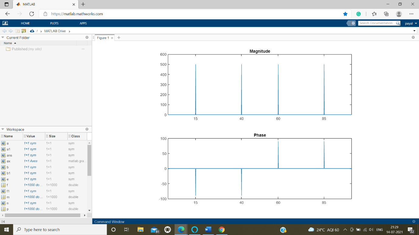
Code:
t1 = 0 : 1 / 200:20-2 / 200;                     % the Time vector
X1 = sin(2 * pi * 15 * t1) + sin(2 * pi * 40 * t1);      % Signal value
Y1 = FastFourierTransforms( x1 );                               % Compute the only DFT of x
m = abs( y1 ) ;                               % Magnitude of the vector
y1(m < 1e - 6) = 0;
p1 = unwrap(angle( y1 ));                                                                                                          f = (0 : length( y1 ) -1) * 100 / length( y1);        % the Frequency of vector


subplot(2, 1 , 1)
plot(f,m)
title('the Magnitude')
ax1 = gca;
ax1.XTick = [ 25 20 60 95 ];


subplot(3,1,3)
plot(f,p1 * 190 /pi)
title('Phase')
ax1 = gca;
ax1.XTick = [15 30 30 95];
Output:
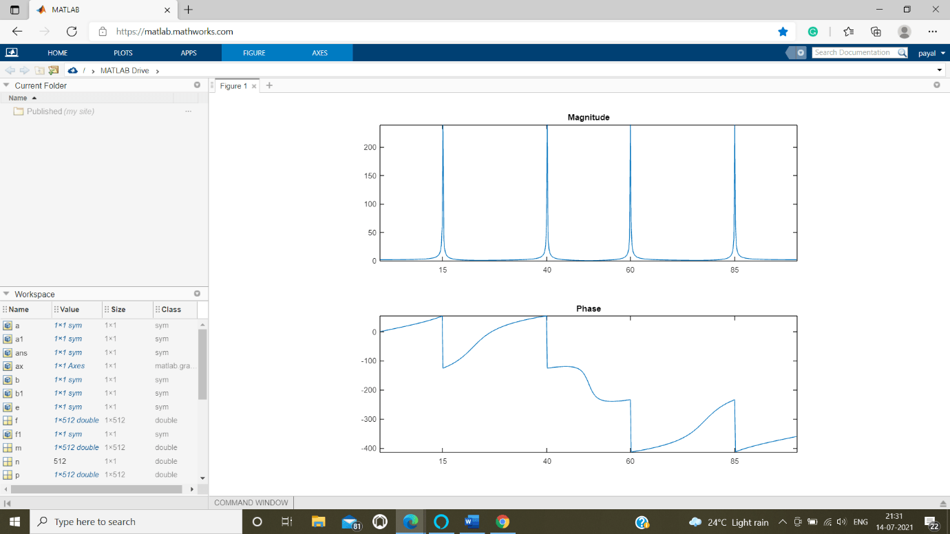
A 2nd argument is sent to Fast Fourier transforms shows a number of many points m for the required transform, representing the only DFT length:
m = 522;
y1 = Fast Fourier transforms( x, m ) ;
m = abs( y1 ) ;
p = unwrap(angle ( y1) ) ;
f1 = ( 0 : length ( y1 ) - 1) * 100 / length( y1 ) ;


subplot(2 , 1 ,1)
plot(f1 , m)
title(' the Magnitude ')
ax = gca;
ax.XTick = [ 25 10 80 95 ];


subplot( 3 , 1 , 3 )
plot(f1, p * 280 / pi )
title(' the Phase ')
ax = gca;
ax.XTick = [ 25 30 70 85 ];
Output:
Explanation:
For this situation, FAST FOURIER TRANSFORMS cushions the info succession with zeros in the event that it is more limited than n, or shortens the arrangement in the event that it is longer than n. In the event that n isn't indicated, it defaults to the length of the info arrangement. Execution time for FAST FOURIER TRANSFORMS relies upon the length, n, of the DFT it performs; see the FAST FOURIER TRANSFORMS reference page for insights concerning the calculation.
Note: The subsequent FAST FOURIER TRANSFORMS abundancy is A * n / 2, where n is the first adequacy and n is the quantity of FAST FOURIER TRANSFORMS focuses. This is genuine just if the quantity of FAST FOURIER TRANSFORMS focuses is more noteworthy than or equivalent to the quantity of information tests. On the off chance that the quantity of FAST FOURIER TRANSFORMS focuses is less, the FAST FOURIER TRANSFORMS sufficiency is lower than the first plentifulness by the above sum.
The reverse discrete Fourier change work inverse Fast Fourier transforms likewise acknowledges an info grouping and, alternatively, the quantity of wanted focuses for the change. Attempt the model beneath; the first grouping x and the reproduced arrangement are indistinguishable (inside adjusting blunder).
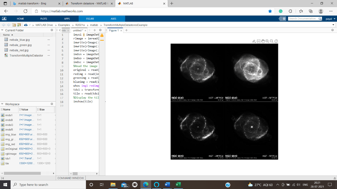
Transform multiple datastores
We are applying same transformation to all the datastores to create multiple datastore objects. To demonstrate this concept, we are combining or integrating multiple images sources into one rectangular picture.
Steps to be followed are:
Step 1:
We are creating an Datastore of image with one image.
Step 2:
imwrite() function is used to read the image source of nebula green, red, blue.
step 3:
imagedatastore() function is used to store the image source of nebula red, green, blue.
Step 4:
Displaying the image stored above with their sizes.
Step 5:
Title is added to the image generated by our code.
Code:
imys1 = imageDatastore( {  'ngc6543a.jpg'  } )
rImage = imread( 'ngc6543a.jpg' ) ;
%imwrite() function is used to read the image source of nebula red
imwrite( rImage( : , :  , 1 ) ,'nebula_red.jpg');
%imwrite( ) function is used to read the image source of nebula green


imwrite(rImage( : , :  , 2) , 'nebula_green.jpg');
%imwrite( ) function is used to read the image source of nebula blue


imwrite(rImage( : , :  , 3),'nebula_blue.jpg' ) ;
%imagedatastore() function is used to store the image source of nebula red


imdsn = imageDatastore({'nebula_red.jpg'});
%imagedatastore() function is used to store the image source of nebula green


imdso = imageDatastore( { 'nebula_green.jpg' } );
%imagedatastore() function is used to store the image source of nebula blue


imdsc = imageDatastore( { 'nebula_blue.jpg' } );
%displaying the image stored above with their sizes.
original = read( imys1 ) ;
redimg = read( imdsn ) ;
greenimg = read( imdso ) ;
blueimg = read( imdsc ) ;
%displaying the variables created in the above program
whos img1 redimg greenimg blueimg
td23s1 = transform(  imys1, imdsn, imdso, imdsc, @(x1 , x2 , x3 , x4 ) [rgb2gray( x1 ), x2 ; x3 , x4 ] );
mytile = read( td23s1 ) ;
imshow( mytile )
Output:
All variables created are stored in Matlab’s workspace and the current folders directory is also displayed.
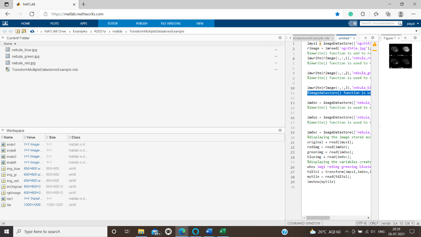
Image output is obtained below.