matlab Integral
What is integration?
In maths, Integral allots numbers to functions in a manner that portrays relocation, region, volume, and different ideas that emerge by consolidating tiny information. The way toward discovering integrals is called integration.
What role it plays in mathematics?
Alongside differentiation, integration is a central, fundamental activity of calculus, and fills in as an apparatus to tackle issues in math and physical science including the space of a self-assertive shape, the length of a bend, and the volume of a strong, among others.
The integrals identified here are those named clear integrals, which can be deciphered officially as the marked space of the district in the plane that is limited by the diagram of a given function capacity between two focuses in the genuine line. Traditionally, regions over the flat graph of the plane are positive while regions breadth are negative. Integrals likewise allude to the idea of an antiderivative, a capacity whose subordinate is the given capacity. For this situation, they are called endless integrals. The crucial hypothesis of calculus relates distinct integrals with differentiation and gives a strategy to register the unmistakable necessary of a capacity when its antiderivative is known.

Matlab Integration
Integration manages two basically various kinds of problems.
- In the main kind, derivative of a function is given and we need to discover the function. In this way, we fundamentally switch the interaction of differentiation. This opposite cycle is known as hostile to separation, or tracking down the crude capacity, or tracking down an indefinite integral.
- The second kind of problem include including an exceptionally enormous number of minuscule amounts and afterward accepting a breaking point as the size of the amounts approaches zero, while the quantity of terms keep an eye on boundlessness. This interaction prompts the meaning of the definite integral
Clear integrals are utilized for discovering region, volume, focus of gravity, snapshot of latency, work done by a power, and in various different applications.
Indefinite Integral in MATLAB
By the given formal definition, if the function f1(x) and it’s derivative is f1'(x), then we declare that f1'(y) an indefinite integral related to y is f(y). For instance, since the obtained derivative (with respect to y) of y4 is as shown 4y, we can declare that an of 4y indefinite integral is y4.
In symbols -
F1'(y4) = 4y, therefore,
? 4ydy = y4.
Example 1
Create a script file code and run through command prompt.
syms y m
int(cos(y))
int(exp(y))
int(log(y))
int(y ^ -1)
int(y ^ 6 * cos(6 * y))
pretty(int(y ^ 6 * cos(6*y)))


int(y ^ - 6)
int(sec(y) ^ 2)
pretty(int(1 – 10 * y + 9 * y^2))


int((3 + 6 * y -6 * y ^ 2 – 7 * y ^ 3)/2 * y ^ 6)
pretty(int((3 + 6 *y -6 * x^2 – 7 * y^3)/6 * y ^ 2))
Output:
ans =

sin(y)


ans =

exp(y)


ans =

y * (log( y ) - 1)


ans =

log(y)


ans =

(5 * y * cos(6 * y )) / 324 - (5 * sin(6 * y))/1944 - (5 * y ^ 3 * cos(6 * y ))/ 54 + (y ^ 5 * cos(6*y))/6 + (5* y ^ 2 * sin(6 * y))/108 - (5 * y ^ 4 * sin(6 * y))/36 + (y ^ 6 * sin(6 * y )) / 6

                             3               5             2               4               6
y cos(6 y) 5   sin(6 y) 5   y  cos(6 y) 5   y  cos(6 y)   y  sin(6 y) 5   y  sin(6 y) 5   y  sin(6 y)
------------ - ---------- - ------------- + ----------- + ------------- - ------------- + -----------
     324          1944            54             6             108              36             6


ans =

-1/(5*y^5)


ans =

tan(y)

      2
y (3 y  - 5 y + 1)


ans =

- (7 * y ^ 10)/20 – y ^ 9/3 + (3 * y ^ 8)/8 + (3 * y ^ 7)/14

   2       2      3
x y  (- 2 x  - 7 y  + 6 y + 3)
------------------------------
               6
Note:
The pretty() function returns an defined labelled expression in a more understandable format.
Example 2:
Indefinite integrals are defined without any given or mentioned limits and containing any arbitrary constant.
Step 1: we use Inline () function for integration function creation.
%we are creating an  inline() function
F1=inline('x ^ 3 + 4 * x' ,'x');
G1=inline( 'sin(y) + cos(y)^3', 'y');
Step 2: Create a symbolic function.
% we are creating a symbolic() function
syms x1;
syms y1;
Step 3: Use int to find out the integration.
% for the integration we kind of use function int()
% and pass the arguments
% (any_expression, any  variable)
% any variable= variable name for the function integration
p=int (f1(x1),x1);
q=int (g1(y1),y1);
Step4: Consolidated code and Output on Matlab’s command prompt:
%we are creating an  inline() function
f1=inline('x ^ 3 + 4 * x' ,'x');
g1=inline( 'sin(y) + cos(y) ^ 3', 'y');
%Step 2: Create a symbolic function.
% we are creating a symbolic() function
syms x1;
syms y1;
%Step 3: Use int to find out the integration.
% for the integration we kind of use function int()
% and pass the arguments
% (any_expression, any  variable)
% any variable= variable name for the function integration
p=int (f1( x1 ), x1);
q=int ( g1(y1) , y1);


p

p =

(x1 ^ 2 * ( x1 ^ 2 + 8))/4

q

q =

sin(y1) - sin(y1 ) ^ 3 / 3 + 2 * sin(y1/ 2) ^ 2

 % (any_expression, any  variable)
Definite Integral in MATLAB
Definite integral is essentially the restriction of an entirety. We utilize positive integrals to discover regions like the region between a bend and the x-axis and the region between two curve bends. Positive integrals can likewise be utilized in different circumstances, where the amount required can be communicated as the constraint of an entirety.
The int() function for definite integration can be used by sending the limits over to which we want to compute the integral.
To calculate we can write,
int(y, a1, b1)For instance, to compute the value of function we write -
int(y, 4, 9)MATLAB executes and returns as follows-
ans =
   65 / 2
Example 1
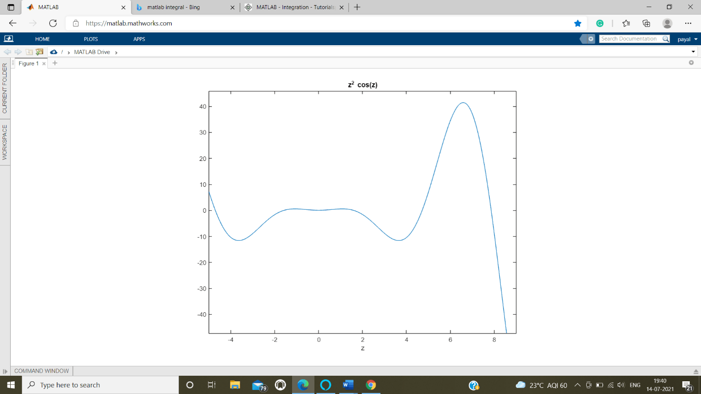
Find the area under the curve: f1(z) = z2 cos(z) for -5 = z = 9.
Create a script file code and run through command prompt.
syms z1
f1 = z1 ^ 2 * cos( z1 );
ezplot(f1 , [-5 , 9 ])
a1 = int( f1, -5, 9)
disp('the Area is as follows: '), disp(double(a1));
When you run the file, MATLAB plots the graph -
Output result:
a1 =

10 * cos (5) + 18 * cos( 9 ) + 23 * sin(5) + 79 * sin(9)

Area is as follows:
   -3.0616
Example 2:
In this instance, we will take a function of degree 3, simple polynomial and will try to integrate it in the limits 0 to 5. We will complete this task in the following 4 steps:
Step 1: create symbols used in the function that is k.
Step2: To perform integration we create degree 3 function in MATLAB environment.
Step 3: Use the function to call it and pass argument to calculate the integration of values.
Step 4: we get the desired output after the code is executed.
Code:
syms k
[the variable ‘k’ is therefore initialized] Gx = @(k) 5 * k.^ 3
[defining the polynomial function of degree 3] A = integral (Gk, 0, 5)
[Passing input argument to the function ‘Gx’ and the required limits to the ‘integral function’] [Statiscally, the integral of 5 * k ^ 3, between the limits 0 to 5 is 95.4333]
Output:
Gk =
@(k) 5 * k. ^ 3
A = 95.4333
Explanation: As we can observe in our desired output, we have obtained integral of our input argument function ‘Gk’ as 95.4333 using predefined ‘integral function’, which is the same as expected output by the user like us.