MATLAB Operators
What is an Operator?
A specific operation is performed by using a symbol which is called an operator.
Example: A+B, where A, B are called operand and '+' is called operator.
If you want to add any two numbers, we will use the '+' symbol, which is nothing but a plus operator. And if you want to divide any two numbers, we use the '/' symbol, division operator.
MATLAB Operators
In MATLAB, all the operators work both on non-scalar and scalar data. MATLAB offers five categories of operators.
Types of operators:
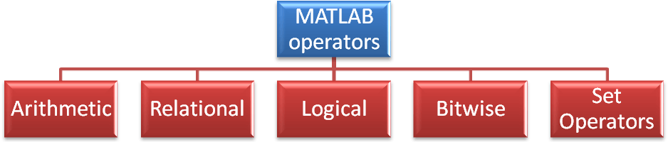
Arithmetic Operators
Arithmetic operators include functions like summation, multiplication, modulo operations, rounding, power, subtraction, differences and approximate derivatives.
- +
Symbol= +, corresponding function=plus(), role=Addition
Syntax à C = A+B or C=plus(A,B)
- +
Symbol= +, corresponding function=uplus(), role=unary plus
Syntax à C = A+B or C=uplus(A,B)
- –
Symbol= -, corresponding function=minus(), role=subtraction
Syntax à C = A-B or C=minus(A,B)
- –
Symbol= -, corresponding function=uminus(), role=unary minus
Syntax à C = A-B or C=uminus(A,B)
- *
Symbol= *, corresponding function=mtimes(), role=matrix multiplication
Syntaxà C=A*B, here A, B are matrix or C=mtimes(A,B)
- .*
Symbol= .* , corresponding function=times(), role=element-wise multiplication
Syntax àC=A.*B or C= times(A,B)
- \
Symbol= \ , corresponding function=mldivide(), role=matrix left division
Syntax à C = A\B or C=mldivide(A,B)
- .\
Symbol= .\, corresponding function=ldivide(), role=element-wise left division
Syntax à C = A.\B or C=ldivide(A,B)
- /
Symbol= /, corresponding function=mrdivide(), role=matrix right division
Syntax à C = A/B or C=mrdivide(A,B)
- ./
Symbol= ./, corresponding function=rdivide(), role=element-wise right division
Syntax à C = A./B or C=rdivide(A,B)
- ^
Symbol= ^, corresponding function=mpower(), role=matrix power
Syntax àC = A^B or C=mpower(A,B)
- .^
Symbol=.^ ,corresponding function=power(), role=element-wise power
Syntax àC = A.^B or C = power(A,B)
- ‘
Symbol=‘ ,corresponding function=ctranspose(), role=complex conjugate transpose
Syntax àB = A’ or B= ctranspose(A)
- .’
Symbol= .’, corresponding function=transpose(), role=transpose
Syntax àB=A.’ or B = transpose(A)
Example:
We have created a script file which has few of the arithmetic operations implemented.
%arithmetic addition is performed
O = [0 1; 1 0];
C = O + 2
%arithmetic subtraction is performed
A = [2 1; 3 5];
D = A-2
%arithmetic multiplication is performed
q = [1 3 5; 2 4 7];
p = [-5 8 1; 3 9 21; 4 0 8];
f = q*p
%arithmetic division is performed
q1 = [1 1 3; 2 0 4; -1 6 -1];
p1 = [2 19 8];
g = p1/q1
%arithmetic power is performed
q2= [1 2; 3 4];
h = q2^2
%arithmetic transpose is performed
B = [2 1; 9 7; 2 8; 3 5]
J = B'
If we run this above script file we are going to obtain the following output.
Expected Output:
C =
2 3
3 2
D =
0 -1
1 3
f =
24 35 104
30 52 142
g =
1.0000 2.0000 3.0000
h =
7 10
15 22
B =
2 1
9 7
2 8
3 5
J =
2 9 2 3
1 7 8 5
Relational Operators
In MATLAB, Relational operators works on both scalar and non-scalar data. These operators mostly return true or false based on result of operation.
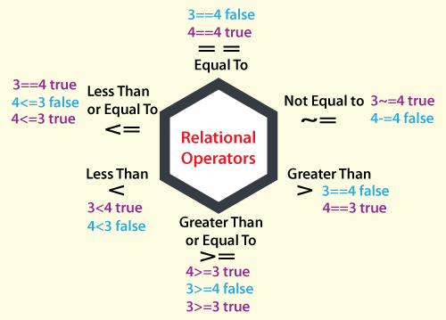
| SYMBOL | Purpose |
| == | EQUAL TO |
| ~= | NOT EQUAL TO |
| > | GREATER THAN |
| >= | GREATER THAN OR EQUAL TO |
| < | LESS THAN IT |
| <= | LESS THAN OR EQUAL TO |
Example:
We have created a script file which has few of the relational operations implemented.
%relational operator "==" is used to check weather matrix q and p are equal
%or not
q = [1+i 3 2 4+i];
p = [1 3+i 2 4+i];
q == p
%Create a duration array and check the condition with relational operator ">=".
f = hours(21:25) + minutes(75)
f >= 1
%Create a array and check the condition with relational operator ">".
w = [1 7 9 11 2 15];
w > 10
%Create array and check the condition with relational operator "<=".
e = [1 7 9 11 2 15];
e <= 12
%Create a array and check the condition with relational operator "<".
d = [1 7 9 11 2 15];
d < 12
%Create g and j arrays, check the condition with relational operator "~=".
g = [1+i 3 2 4+i];
j = [1 3+i 2 4+i];
g ~= j
%Create q1 and p1 matrices to check the condition with relational operator "isequal()".
q1 = zeros(3,3)+1e-20;
p1 = zeros(3,3);
f1 = isequal(q,p1)
If we run this above script file we are going to obtain the following output.
ExpectedOutput:
ans =
1×4 logical array
0 0 1 1
f =
1×5 duration array
22.25 hr 23.25 hr 24.25 hr 25.25 hr 26.25 hr
ans =
1×5 logical array
0 0 1 1 1
ans =
1×6 logical array
0 0 0 1 0 1
ans =
1×6 logical array
1 1 1 1 1 0
ans =
1×6 logical array
1 1 1 1 1 0
ans =
1×4 logical array
1 1 0 0
f1 =
logical
0
30 52 14
Logical Operators
Onlytwological operators are available in MATLAB.
- Element-wise
This type of operator works only on logical arrays.
| Symbol | Description |
| & | Logical AND |
| ~ | Logical NOT |
| | | Logical OR |
- Short-circuit
There are two short-circuit logical operators which work on both the operations, scalar and logical.
| Symbol | Description |
| || | Logical OR (short-circuit) |
| && | Logical AND (short-circuit) |
Example:
We have created a script file which has few of the logical operations implemented.
%And operation of matrix q and p.
q = [5 7 0; 0 2 9; 5 0 0]
p = [6 6 0; 1 3 5; -1 0 0]
q & p
%Logical negation of q.
q1 = eye(3)
p1 = ~q1
%Logical or operations of matrix q and p.
q2 = [5 7 0; 0 2 9; 5 0 0]
p2 = [6 6 0; 1 3 5; -1 0 0]
q2 | p2
%Xor operation of q.
q3 = [true false]
p3 = [true; false]
C = xor(q3,p3)
So, you can simply copy this file and run in your MATLAB software. If we run this above script file we are going to obtain the following output.
Expected output:
q =
5 7 0
0 2 9
5 0 0
p =
6 6 0
1 3 5
-1 0 0
ans =
3×3 logical array
1 1 0
0 1 1
1 0 0
q1 =
1 0 0
0 1 0
0 0 1
p1 =
3×3 logical array
0 1 1
1 0 1
1 1 0
q2 =
5 7 0
0 2 9
5 0 0
p2 =
6 6 0
1 3 5
-1 0 0
ans =
3×3 logical array
1 1 0
1 1 1
1 0 0
q3 =
1×2 logical array
1 0
p3 =
2×1 logical array
1
0
C =
2×2 logical array
0 1
1 0
30 52 14
Bitwise Operators
As the name suggests that these operators work on bit-by-bit operations.
The truth table involved in this operation is as follows.
| H | K | h&k | h|k | h^k |
| 0 | 0 | 0 | 0 | 0 |
| 0 | 1 | 0 | 1 | 1 |
| 1 | 1 | 1 | 1 | 0 |
| 1 | 0 | 0 | 1 | 1 |
Various MATLAB bitwise functions are as follows.
- bitand(g,h)à Bit-wise AND
- bitor(g,h)à Bit-wise OR
- bitcmp(g)à Bit-wise COMPLEMENT
- bitxor(g,h)à Bit-wise XOR
- bitget(g,pos)à Bit-wise to get position of a
- bitset(g,pos)à Bit-wise to set position of a
- bitShift(g,k)à Bit-wise SHIFT
Let us execute these bitwise functions in MATLAB’s command line and see how itresults.
>>g=34
g =
34
>>h=7
h =
7
>>bitand(g,h)
ans =
2
>>bitor(g,h)
ans =
39
>bitxor(g,h)
ans =
37
>>bitcmp(g)
ans =
1.8447e+19
>>bitget(g,h)
ans =
0
Set Operations
Set operations include testing set membership, union or intersection of two given sets, it resembles set theory of mathematics.
Various MATLAB set operations are as follows.
- intersect(A,B)
- intersect(A,B,’rows’)
- ismember(A,B)
- ismember(A,B,’rows’)
- issorted(A)
- issorted(A,’rows’)
- setdiff(A,B)
- setdiff(A,B,’rows’)
- setxor(A,B)
- union(A,B)
- unique(A)
Let us check out theseset operation functions in MATLAB’s command line.
In the below code, we see two sets: A and B, which are internally created as 1x1 matrix array. We applied all the above-mentioned set operation functions and executed them to get results. The result of each function is reserved in a default variable “ans” created by MATLAB’s environment. Check out the following code.
>>A=[1 6 1 4]
A =
1 6 1 4
>>B=[8 3 6 3]
B =
8 3 6 3
>>intersect(A,B)
ans =
6
>>intersect(A,B,"rows")
ans =
0×4
>>ismember(A,B)
ans =
1×4
0 1 0 0
>>ismember(A,B,"rows")
ans =
logical
0
>>issorted(A)
ans =
logical
0
>>issorted(A,'rows')
ans =
logical
1
>>setdiff(A,B)
ans =
1 4
>>setdiff(A,B,"rows")
ans =
1 6 1 4
>>setxor(A,B)
ans =
1 3 4 8
>>union(A,B)
ans =
1 3 4 6 8
>>unique(A)
ans =
1 4 6
b=7