Linear Regression in R Programming

Linear Regression is an unsupervised machine learning algorithm in R programming. Linear Regression is a type of regression analysis that shows the relationship between two or more variables. And one of these variables is called the predictor variable, and the other is the response variable.

The predictor variable is estimated by using some statistical experiments. The predictor variable is the one whose value is gathered through experiments. And the Responsible variables are the ones whose value is derived from the predictor variable.

Linear Regression is the most used regression technique over all other regression techniques. Linear Regression creates a predictive model using the relevant data to show trends.

Below is the simple equation of Linear Regression,

y = ax+b


Description of the above parameters, 
y = Responsible Variable
a =Coefficients (Constants)
x = Predictor Variable
b = Coefficients (Constants)

The linear regression graph is plotted as a straight line, as shown below.

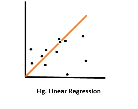
This is the simplest plot of linear regression. That orange line represents a linear regression. And the black dots represent the data points.

Let's take the example of linear regression to understand the topic better. A very simple example of linear regression can be the height and weight of a student. A student's height is already known to us, and we have to predict a student's weight.

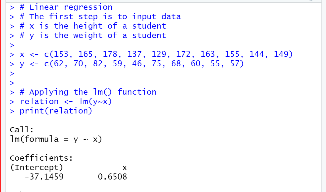
The first step is to gather a sample of observed values of a height and the corresponding weight of the student. Then by using the built-in lm() function R, we will create a relationship model. After that, we will find the coefficients from the above model and create the mathematical equations using all the information.

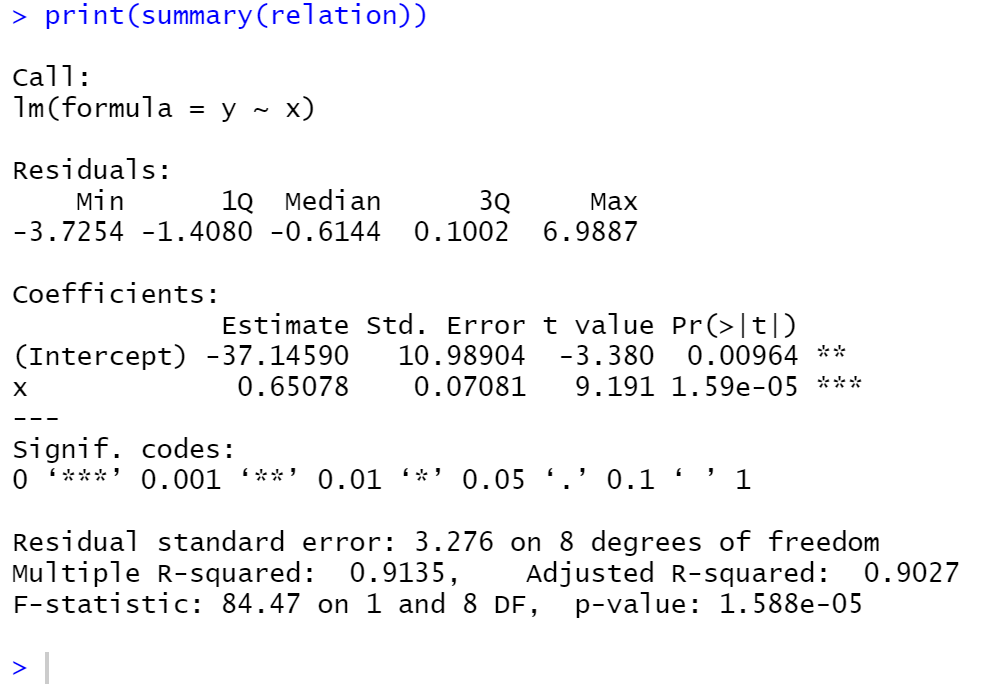
Once we are done with the equation, we will get the summary of our relationship model to know the average error in the prediction, which can also be termed residuals. And at the end, to predict the weight of a new student, we will use the predict() function.

INPUT DATA:

HEIGHT	WEIGHT
153	62
165	70
178	82
137	59
129	46
172	75
163	68
155	60
144	55
149	57

CODE:

# Linear regression
# The first step is to input data 
# x is the height of a student
# y is the weight of a student


x <- c(153, 165, 178, 137, 129, 172, 163, 155, 144, 149)
y <- c(62, 70, 82, 59, 46, 75, 68, 60, 55, 57)
  


# Applying the lm() function
relation <- lm(y~x)
print(relation)

When we try to execute the above code in R studio, we get the output as:

OUTPUT:

Now, we will get the summary of our relationship mode and use print(summary(relation)).

CODE:

x <- c(153, 165, 178, 137, 129, 172, 163, 155, 144, 149)
y <- c(62, 70, 82, 59, 46, 75, 68, 60, 55, 57)
  


# Applying the lm() function
relation <- lm(y~x)
print(relation)


# Finding Relationship:
print(summary(relation))

OUTPUT:

predict() function:

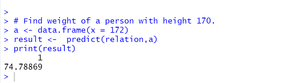
We are using predict function to predict the weight of the new student.

Syntax of predict() function:

predict(object, newdata)


Where, 


object – formula (already created using lm() function)
new data – vector containing new values 

CODE:

# Linear regression
# The first step is to input data 
# x is the height of a student
# y is the weight of a student


x <- c(153, 165, 178, 137, 129, 172, 163, 155, 144, 149)
y <- c(62, 70, 82, 59, 46, 75, 68, 60, 55, 57)
  


# Applying the lm() function
relation <- lm(y~x)
print(relation)


# Here we are finding weight of a student with height 172.
a <- data.frame(x = 172)
result <-  predict(relation,a)
print(result)

When we try to execute the above code in R studio, we get the following result:

OUTPUT:

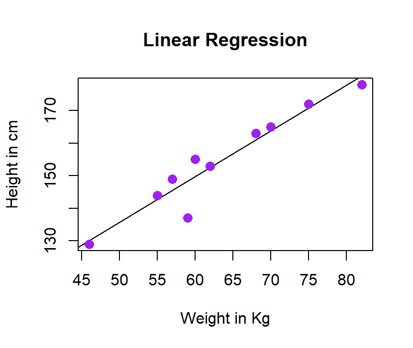
Visualizing the Regression:

The last step which is left to perform is visualizing the regression graphically.

CODE:

# Linear regression
# The first step is to input data 
# x is the height of a student
# y is the weight of a student


x <- c(153, 165, 178, 137, 129, 172, 163, 155, 144, 149)
y <- c(62, 70, 82, 59, 46, 75, 68, 60, 55, 57)




# Applying the lm() function
relation <- lm(y~x)
print(relation)


# Visualizing the graph
# Plot the chart.
plot(y,x,col = "purple",main = "Linear Regression",
     abline(lm(x~y)),cex = 1.3,pch = 16,xlab = "Weight in Kg",ylab = "Height in cm")

When we try to execute the above code in r studio, we get the following result:

OUTPUT:

Conclusion:

We can conclude that linear regression is very simple, easy to understand, and easy to fit, yet it is a very powerful model. This article taught us how to perform linear regression model analysis on R. This was all about linear regression in R programming.