Logistic Regression in R Programming

Logistic Regression is a classification supervised machine learning algorithm in R programming. Logistic Regression can also be termed Binomial Logistic Regression, Binary Logistic Regression, or Logit Model. Logistic Regression is a Generalized Linear Model. Logistic Regression classifies binary or multi-class data values. So, with the help of logistic Regression, we can build a model which segregates and classify binary data values.

Logistic Regression is mostly used when we have to find the probability of the event’s success and failure. Logistic Regression is another type of regression model where the dependent variable (response variable) has categorical values, namely 0/1, True/False, or Yes/No.

Logistic Regression measures the probability of binary response as the value of the dependent or response variable is based on the mathematical equation relating to it with the predictor variables.

Logistic Regression works on the logit function; this function segregates the binary labeled values in our dataset. In a binomial distribution, the logit function is used as a link function.

Logistic Regression is based on the sigmoid function. The reason is that the input can be anything from -infinity to + infinity, but the output is probability. So it has to be between 0 to 1.

Now, let’s have a look at the simplest Logistic Regression equation:

y = 1/(1+e^-(a+b1x1+b2x2+b3x3+………+bnxn))


Description of the above parameters:


y = response variable (dependent variable)
a = coefficients (constant)
b = coefficients (constant)
x = predictor variable

As we know, the Regression model is created using the glm() function. So the basic syntax of the glm() function is as follows:

SYNTAX:

glm(formula, data, family)


Description of the above parameters:


glm - generalized linear model
formula – formula represents the relationship between the variables
data - data is the dataset that gives the values of these variables
family – It is an R object specifying the details of our model. The value of the R object is binomial for logistic regression. 

Let’s have a look at one example to have a better understanding of the topic:

CODE:

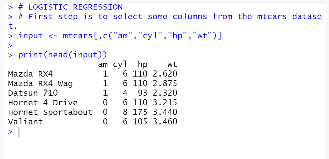
# LOGISTIC REGRESSION
# First step is to select some columns from the mtcars dataset.
input <- mtcars[,c("am","cyl","hp","wt")]


# head is used to print the first part of any vector, dataframe, or matrix.
print(head(input))

By executing the above code in RStudio, the following result is produced:

OUTPUT:

CREATING REGRESSION MODEL:

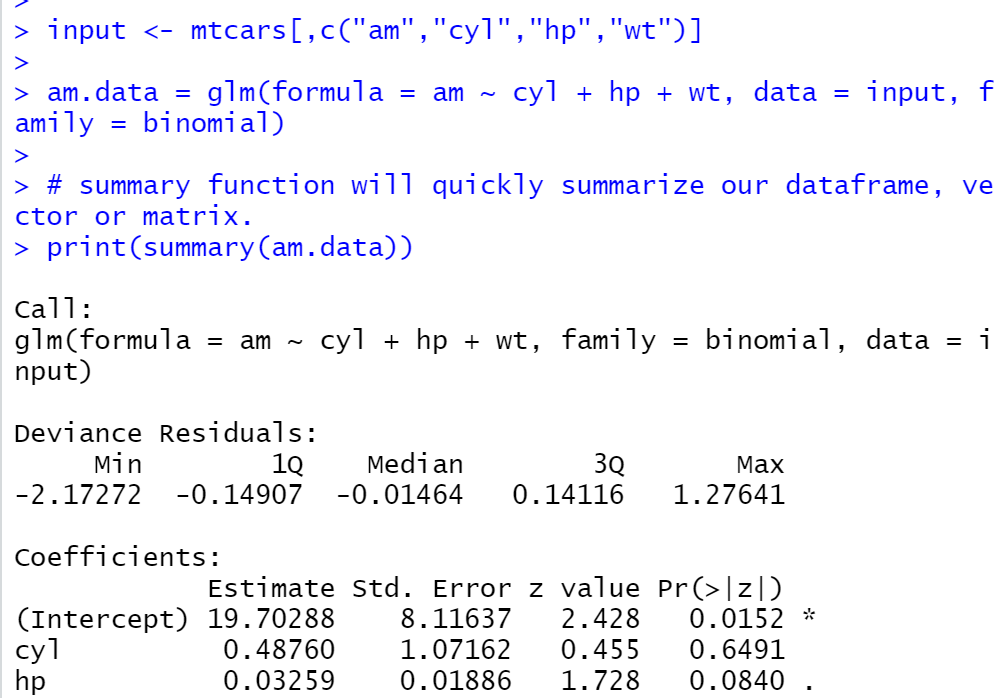
Using the glm() function, we will create a Regression model and get the summary of our model for analysis.

CODE:

# LOGISTIC REGRESSION
# First step is to select some columns from the mtcars dataset.
input <- mtcars[,c("am","cyl","hp","wt")]


# head is used to print the first part of any vector, dataframe, or matrix.
print(head(input))


input <- mtcars[,c("am","cyl","hp","wt")]


am.data = glm(formula = am ~ cyl + hp + wt, data = input, family = binomial)


# summary function will quickly summarize our dataframe, vector or matrix. 
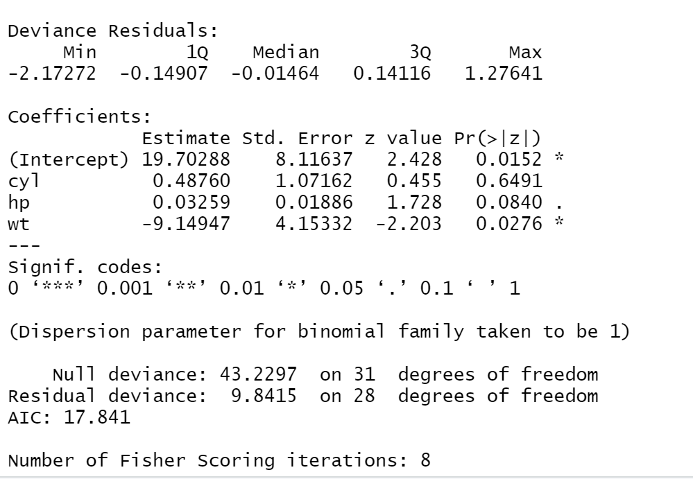
print(summary(am.data))

By executing the above code in RStudio, the following result is produced:

OUTPUT:

HOW TO PLOT A LOGISTIC REGRESSION CURVE IN R PROGRAMMING?

There are 2 methods of creating a Logistic Regression curve in R programming. They are as follows:

1. Base R Methods
2. ggplot2 Package

a) Base R Methods:

• The first step is to fit the variables in the Logistic Regression model using the glm() function.
• Then, we will create a dataframe where the variables of the y-axis are changed to their predicted variable by using predict() function.
• After that, we will create a scatter plot using the plot() function and predicted values using the lines() function.

SYNTAX:

# Logistic Model
glm(formula, family, dataframe)


# Plotting original dataframe
plot(o_dataframe)


# Plotting predicted dataframe
lines(p_dataframe)

EXAMPLE 1:

CODE:

# Fitting Logistic Regression Model
model <- glm(vs ~ wt, data=mtcars, family=binomial)


# Defining new data frame which contains predictor variable
newdata <- data.frame(wt=seq(min(mtcars$wt), max(mtcars$wt),len=500))


# Using fitted model to predict the values of vs
newdata$vs = predict(model, newdata, type="response")


# Plotting logistic regression curve
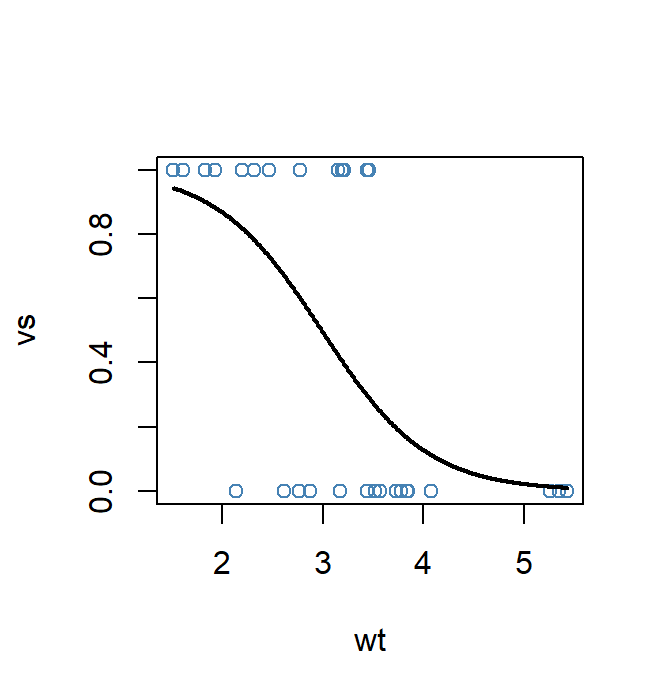
plot(vs ~ wt, data=mtcars, col="steelblue")
lines(vs ~ wt, newdata, lwd=2)

By executing the above code in RStudio, the following result is produced:

OUTPUT:

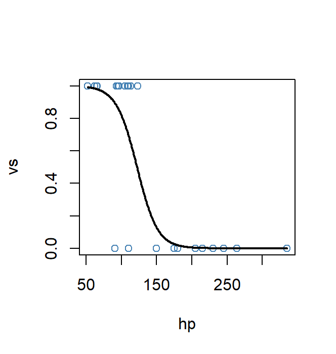
EXAMPLE 2:

CODE:

# Fitting Logistic Regression Model
model <- glm(vs ~ hp, data=mtcars, family=binomial)


# Defining new data frame which contains predictor variable
newdata <- data.frame(hp=seq(min(mtcars$hp), max(mtcars$hp),len=500))


# Using fitted model to predict the values of vs
newdata$vs = predict(model, newdata, type="response")


# Plotting logistic regression curve
plot(vs ~ hp, data=mtcars, col="steelblue")
lines(vs ~ hp, newdata, lwd=2)

By executing the above code in RStudio, the following result is produced:

OUTPUT:

b) ggplot2 Package:

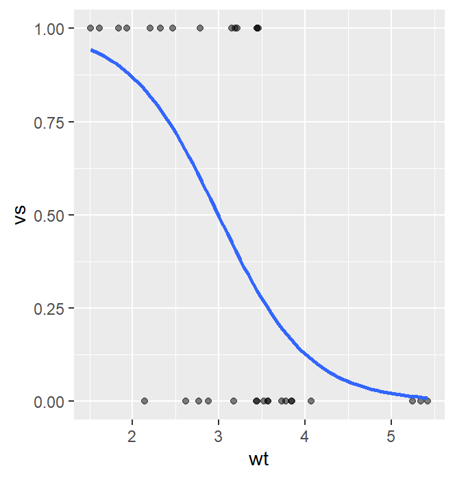
EXAMPLE 1:

CODE:

# Installing ggplot2 library.
library(ggplot2)


# Plotting logistic regression curve.
ggplot(mtcars, aes(x=wt, y=vs)) + 
  geom_point(alpha=.5) +
  stat_smooth(method="glm", se=FALSE, method.args = list(family=binomial))

By executing the above code in RStudio, the following result is produced:

OUTPUT:

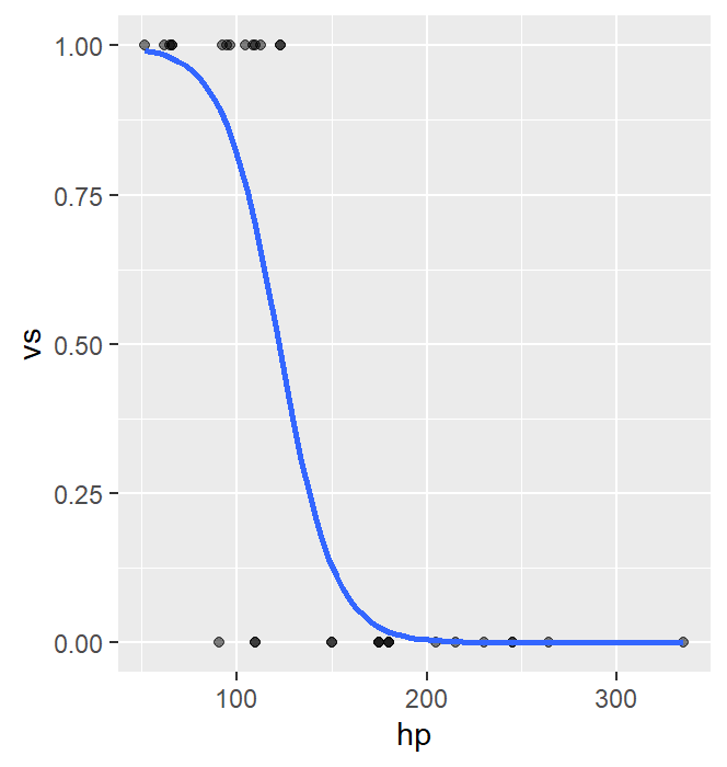
EXAMPLE 2:

CODE:

# Installing ggplot2 library.
library(ggplot2)


# Plotting logistic regression curve.
ggplot(mtcars, aes(x=hp, y=vs)) + 
  geom_point(alpha=.5) +
  stat_smooth(method="glm", se=FALSE, method.args = list(family=binomial))

By executing the above code in RStudio, the following result is produced:

OUTPUT:

CONCLUSION:

So, this was all about Logistic Regression in R Programming. And how to plot the curve of Logistic Regression in RStudio.