Measures of Central Tendency in R Programming

Central Tendency or CT is one of the features of descriptive statistics. The Central tendency will let us know how the various groups of data are clustered around the central value of the distribution of the dataset.

In layman’s terms, the measures of central tendency represent the whole set of data by a single value. And it also gives us the location of the central points of our dataset.

Generally, there are 3 main measures of central tendency. They are as follows:

1. Mean
2. Median
3. Mode

There are 2 more measures of central tendency which are not so common. They are geometric mean and harmonic mean. Let’s discuss a little bit about both mean later.

Let’s understand all the measures of central tendency one by one before jumping toward any computation.

• Mean:
  • The mean is nothing but the average value of our dataset.
  • Mathematically, the mean is the sum of observations (∑X) divided by the total number of observations (n).
  • Mean is denoted by x̄.
  • Syntax of mean is:
    
    Mean(x, trim, na.rm = FALSE)

Mean (x̄) = ∑x

                   n

Where,

x̄ = Mean

∑x = Sum of observations

n = Total number of observations

Example 1:

Illustration of finding mean in R Studio:

# Let's create a vector.
x <- c(1,3,5,7,4,9,2)
result.mean <- mean(x)
print(result.mean)

When executing the above code in R Studio, you get the following output.

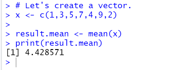
OUTPUT:

Example 2:

Calculating the mean of age in the diabetes dataset.

CODE:

diabetes = read_excel(C:\Users\Dhruvi Patel\Documents\DATASETS\diabetes.xls")
print(diabetes)


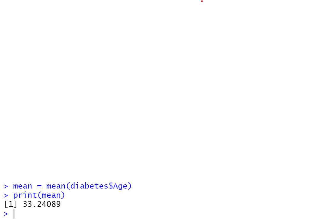
mean = mean(diabetes$Age)
print(mean)

OUTPUT:

[1] 33.24089

• Let’s understand the code first. The first step is to import the dataset into R Studio.
• So, for that, you have to go to import dataset and then select the option From Text (Base)
• Then, select the dataset you want to upload.
• Once you are done selecting the file, just click import.
• This is how you can import any dataset in R studio.
• After that, you have to read the dataset. So, for reading the dataset, you will use the syntax read_file type (“Location of the File\Name of the File\.extension”).
• And then, you will print the dataset.
• And use the syntax of calculating the mean as follows.

CODE:

diabetes = read_excel(“c:\users\Dhruvi Patel\Documents\DATASETS\diabetes.xls”)
print(diabetes)


mean = mean(diabetes$Age)
print(mean)

OUTPUT:

This is how you can calculate the mean in R studio.

• Median:
  • The median is another measure of central tendency.
  • The median is nothing but the middle value of any dataset, i.e., it splits the dataset into 2 halves.
  • Syntax of the median is:
    median(x, na.rm = FALSE)
  • Parameters are:
    x = data vector
    na.rm = If TRUE then it removes the value of NA from x

Example 1:

CODE:

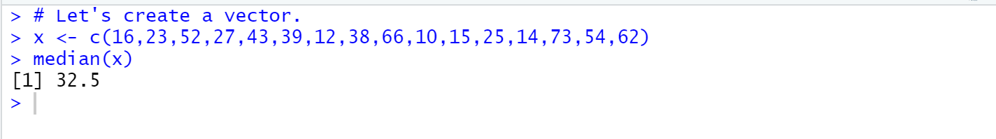
# Let's create a vector.
x <- c(16,23,52,27,43,39,12,38,66,10,15,25,14,73,54,62)
median(x)

OUTPUT:

[1] 32.5

# Let's create a vector.
x <- c(16,23,52,27,43,39,12,38,66,10,15,25,14,73,54,62)
median(x)

OUTPUT:

When we execute the above code, we get the output as:

Example 2:

CODE:

diabetes = read_excel(“c:\users\Dhruvi Patel\Documents\DATASETS\diabetes.xls”)
print(diabetes)


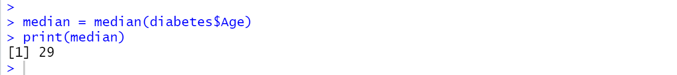
median = median(diabetes$Age)
print(median)

When we execute the above code, we get the output as:

• Mode:
  • Mode is the most frequently occurring number or value in our dataset.
  • There can be a possibility that a dataset has no mode. This only occurs when the frequency of all data points is the same.
  • We can have one or more than one mode in a dataset when two or more than two data points have the same frequency.
  • But there is no built-in function pre-defined in R to find mode.
  • Hence, we can create a function for finding the mode in R, or else we can use the package modest.

Example 1: Single Value Mode

CODE:

# Defining vector
x <- c(13, 27, 51, 43, 28, 21, 44,  
       23, 44, 56, 78, 65, 56,
       23, 44, 44, 37, 45, 71, 44, 98)


y <- table(x)
print(y)


# Mode of x
m <- names(y)[which(y == max(y))]
print(m)

When we execute the above code, the results/output is as follows:

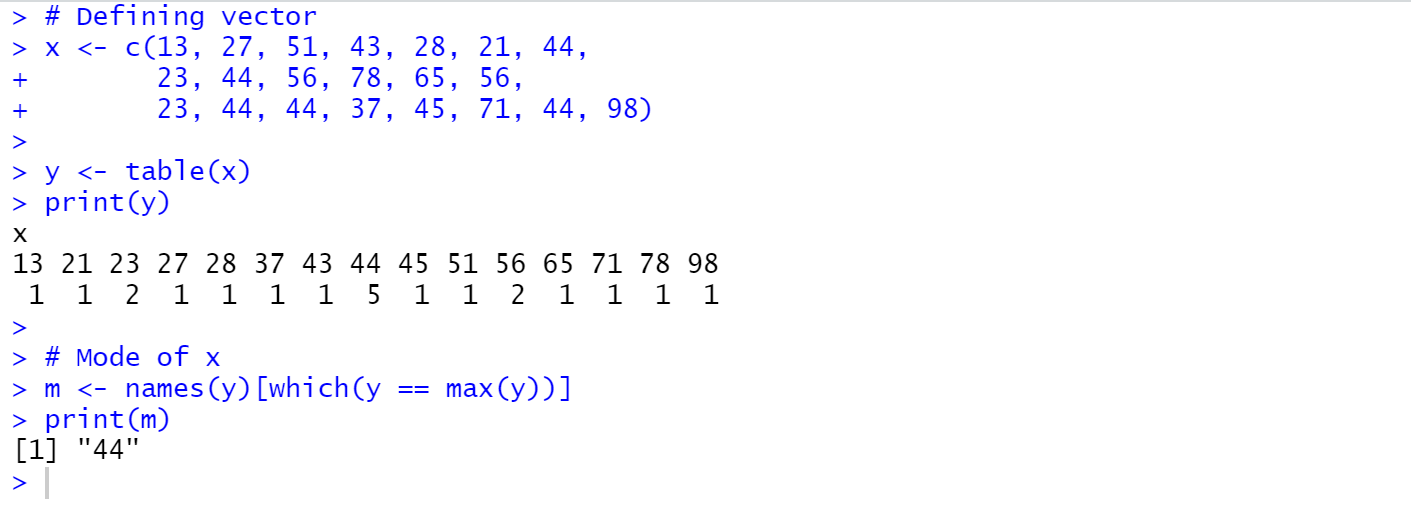
OUTPUT:

[1] "44"

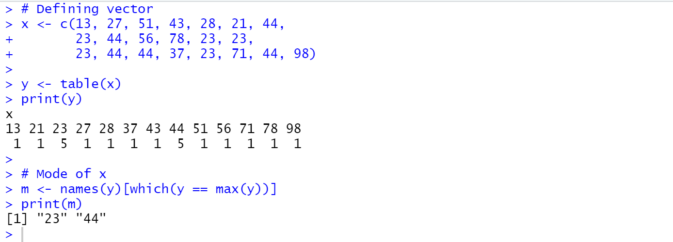
Example 2: Multiple Values Mode

CODE:

# Defining vector
x <- c(13, 27, 51, 43, 28, 21, 44,  
       23, 44, 56, 78, 23, 23,
       23, 44, 44, 37, 23, 71, 44, 98)


y <- table(x)
print(y)


# Mode of x
m <- names(y)[which(y == max(y))]
print(m)

OUTPUT:

[1] "23" "44"

Harmonic Mean:

• Harmonic mean is another type of mean used to compute the reciprocal of the arithmetic mean of reciprocals of the given set of values.
• The syntax of the harmonic mean is:
  (1/mean(1/x))

CODE:

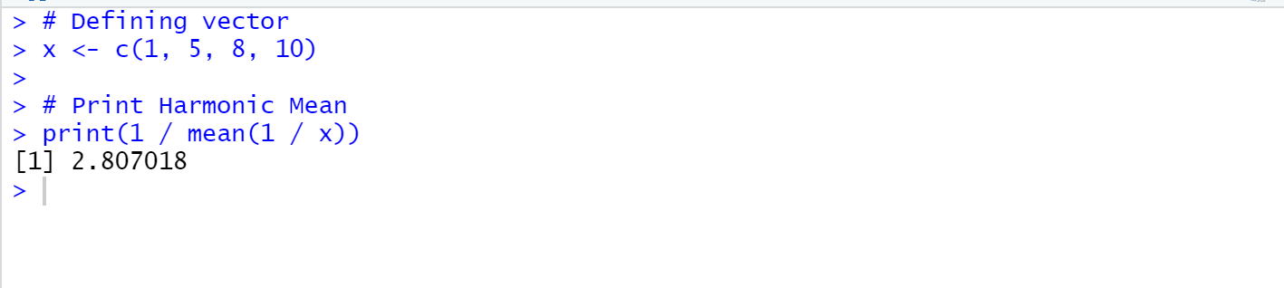
# Defining vector
x <- c(1, 5, 8, 10)


# Print Harmonic Mean
print(1 / mean(1 / x))

OUTPUT:

[1] 2.807018

Geometric Mean:

• This is another type of mean which can be computed by multiplying all the data values.
• Syntax of the geometric mean is:
  prod(x)^(1/length(x)))

where,

x = vector

prod() = it returns the product of all values present in vector x

length() = it returns the length of vector x

Example:

CODE:

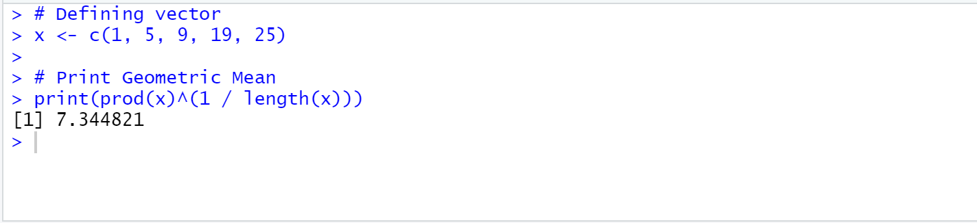
# Defining vector
x <- c(1, 5, 9, 19, 25)
  
# Print Geometric Mean
print(prod(x)^(1 / length(x)))

OUTPUT:

[1] 7.344821

This is what the output looks like when we run the code in R: