Chi-Square Test in Machine Learning
A statistical technique called the chi-square test is used to compare actual outcomes to predictions. This test aims to determine if a discrepancy between actual and projected data is caused by chance or by a connection between the variables being examined. The chi-square test is a great option for helping us comprehend and evaluate the relationship between our two categorical variables as a result.
The distribution of a categorical variable must be tested using a chi-square test or analogous non-parametric test. Nominal or ordinal categorical variables can represent categorical variables like animals or nations. Since they can only have a few specific values, they cannot have a normal distribution.
For instance, the relationship between gender, region, and people's food choices is something that an Indian meal delivery service wants to look into.
It is used to figure out how different two category variables are, namely:
- Due to coincidence
- Considering the relationship
Formula For Chi-Square Test

Here,
c = Degrees of freedom
O = Observed Value
E = Expected Value
The number of variables that can change in a computation is represented by the degrees of freedom in a statistical calculation. It is possible to determine the degrees of freedom to make sure chi-square tests are statistically reliable. These tests are typically employed to contrast the observed data with the data that would be anticipated if a specific hypothesis were to be correct.
The values you collect yourself make up the observed values.
According to the null hypothesis, the values and frequencies are predicted.
What can a Chi-Square Test Tell You?
Fundamentally, a Chi-Square test is a data analysis based on the observations of a diverse range of variables. It computes the relationship between a model and the actual observed data. The data used to construct the Chi-Square statistic test must be unprocessed, random, derived from independent variables, derived from a large sample, and mutually exclusive. In layman's words, two sets of statistical data—for instance, the outcomes of tossing a fair coin—are compared. This test was developed by Karl Pearson in 1900 for the analysis and distribution of categorical data. "Pearson's Chi-Squared Test" is another name for this assessment.
The most typical method for assessing hypotheses for categorical variables is the chi-squared test. A hypothesis is an assertion that may be tested later that any given situation might be true. When the sample size and the number of variables in the relationship are stated, the Chi-Square test calculates the amount of the discrepancy between the predicted and actual findings.
Degrees of freedom are used in these tests to assess whether a certain null hypothesis can be ruled out based on the overall number of observations made during the experiment. The reliability of the finding increases with the sample size.
There are two main types of Chi-Square tests, namely -
- Independence
- Goodness-of-Fit
Independence
A derivable (also known as inferential) statistical test called the Chi-Square Test of Independence determines whether two sets of variables are likely to be connected to one another or not. This non-parametric test is applied when there are counts of values for two nominal or categorical variables. The requirements for carrying out this test are an independent set of observations and a sizable sample size.
For Example:
Imagine we created a list of movie genres for a theatre. This will serve as the initial variable, please. The second factor is whether or not folks who came to the theatre to watch certain types of movies also purchased concessions. The movie's genre and whether or not people bought snacks are here the null hypothesis since they are unrelatable. If this is the case, movie genres have no impact on snack sales.
Let's create some fictitious voter polling data and do an independence test:
np.random.seed(10)


# random data sampling with predetermined probability
race_of_voter = np.random.choice(a= ["asian","black","hispanic","other","white"],
                              p = [0.05, 0.15 ,0.25, 0.05, 0.5],
                              size=1000)


# random data sampling with predetermined probability
party_of_voter = np.random.choice(a= ["democrat","independent","republican"],
                              p = [0.4, 0.2, 0.4],
                              size=1000)


voter = pd.DataFrame({"race":voter_race,
                       "party":voter_party})


tab_of_voter = pd.crosstab(voters.race, voters.party, margins = True)


tab_of_voter.columns = ["democrat","independent","republican","row_totals"]


tab_of_voter.index = ["asian","black","hispanic","other","white","col_totals"]


observation = tab_of_voter.iloc[0:5,0:3]   # Get table without totals
tab_of_voter
Output:
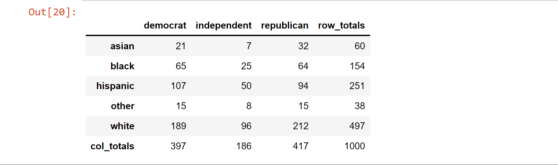
Note: The variables are independent since we did not utilize the race data to help us generate the party data.
By using the table's row and column totals, performing an outer product on them using the np.outer() function, then dividing the result by the number of observations, we can rapidly obtain the predicted counts for all cells in the table:
expectation =  np.outer(tab_of_voter["row_totals"][0:5],
                     tab_of_voter.loc["col_totals"][0:3]) / 1000


expectation = pd.DataFrame(expectation)


expectation.columns = ["democrat","independent","republican"]
expectation.index = ["asian","black","hispanic","other","white"]


expectation
Output:

Calculating the chi-square statistic, the critical value, and the p-value
chi_squared_statistics = (((observation-expectation)**2)/expectation).sum().sum()


print(chi_squared_statistics)
Output:
7.169321280162059
Note: In order to retrieve the total of the complete 2D table, we call.sum() twice: once to obtain the column sums and again to add the column sums.
critical_value = stats.chi2.ppf(q = 0.95, # Finding the critical value for 95% confidence level
                      df = 8)   # *


print("Critical value")
print(critical_value)


p_value = 1 - stats.chi2.cdf(x=chi_squared_statistics,  # Finding the p-value
                             df=8)
print(" ")
print("P value")
print(p_value)
Output:
Critical value
15.50731305586545

P value
0.518479392948842

Scipy allows us to perform an independence test rapidly.
In order to automatically perform an independence test given a frequency table of observed counts, use the stats.chi2 contingency() function:
stats.chi2_contingency(observed= observation)
Output:
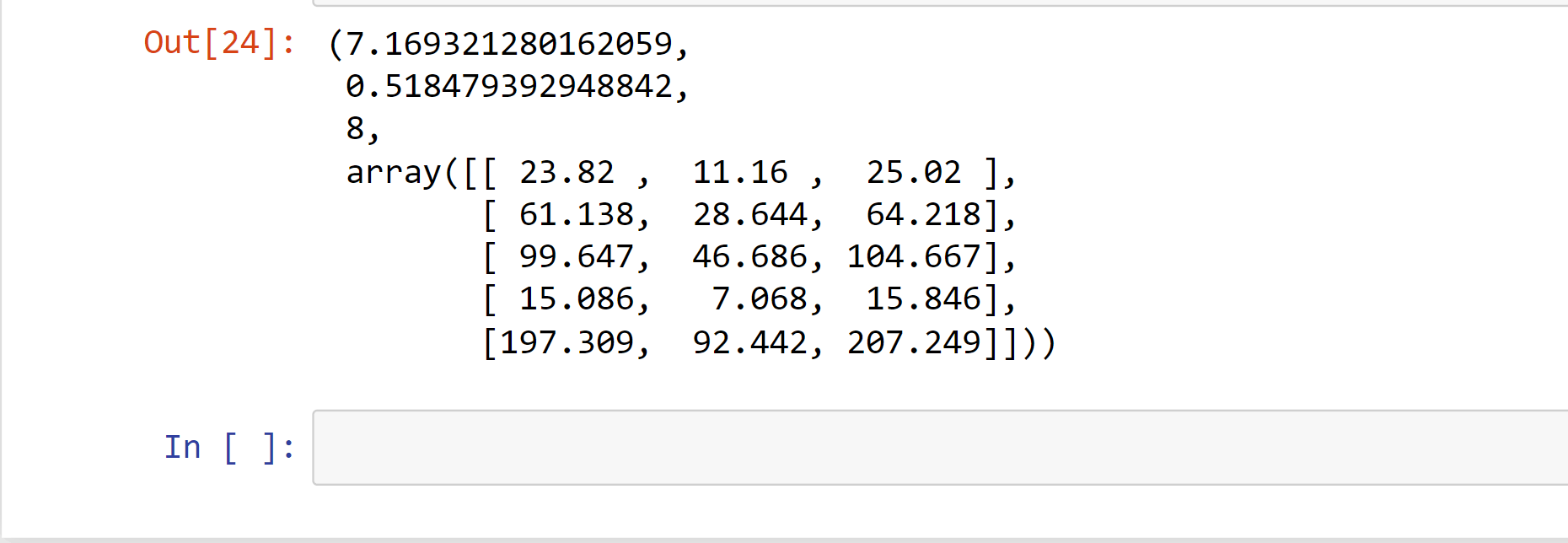
The predicted counts are followed by the chi-square statistic, the p-value, and the degrees of freedom in the output.
The test result did not find a significant association between the variables, as would be expected given the high p-value.
Goodness-Of-Fit
The Chi-Square Goodness-of-Fit test in statistical hypothesis testing examines if a variable is likely to originate from a specific distribution or not. We must have a collection of data values and an understanding of how the data are distributed. When categorical variables contain value counts, we may utilize this test. This test shows how to determine whether the data values have a "good enough" fit for our hypothesis or whether they are a representative sample of the complete population.
For Example:
Consider that each bag of balls has five distinct colors of balls. The requirement is that there must be an equal number of balls in each color in the bag. The notion that the proportions of the five different ball colors in each bag must be precise is what we're trying to test here.
Let's create fictitious demographic data for the United States and Minnesota and run them through the chi-square goodness of fit test to see whether they differ:
# Importing Libraries
import numpy as np
import pandas as pd
import scipy.stats as stats
In_nation = pd.DataFrame(["white"]*100000 + ["hispanic"]*60000 +\
["black"]*50000 + ["asian"]*15000 + ["other"]*35000)
In_minnesota = pd.DataFrame(["white"]*600 + ["hispanic"]*300 + \
["black"]*250 +["asian"]*75 + ["other"]*150)
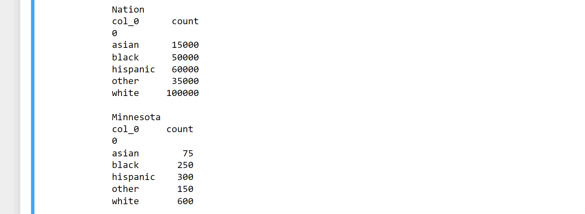
In_national_table = pd.crosstab(index=In_nation[0], columns="count")
In_minnesota_table = pd.crosstab(index=In_minnesota[0], columns="count")
print( "Nation")
print(In_national_table)
print(" ")
print( "Minnesota")
print(In_minnesota_table)
Output:
observation = In_minnesota_table


ratio_of_nation = In_nation_table/len(In_nation)  # Get population ratios


expectation = ratio_of_nation * len(In_minnesota)   # Get expected counts


chi_squared_statistics = (((observation-expectation)**2)/expectation).sum()


print(chi_squared_statistics)
Output:
col_0
count    18.194805
dtype: float64
In the chi-square test, the test statistic is compared to a critical value based on the chi-square distribution. The chi-square distribution is abbreviated as chi2 in the Scipy library.
Using this information, let's calculate the crucial value for a 95% confidence level and get the p-value of our outcome.
critical_value = stats.chi2.ppf(q = 0.95, # Finding the critical value for 95% confidence level
                      df = 4)   # Df = number of variable categories - 1(Degree of Freedom)


print("Critical value")
print(critical_value)


p_value = 1 - stats.chi2.cdf(x=chi_squared_statistics,  # Find the p-value(significant value)
                             df=4)
print("p-value")
print(p_value)
Output:
Critical value
9.487729036781154
p-value
[0.00113047]

Our chi-squared statistic is higher than the threshold. Therefore we can rule out the null hypothesis that the two distributions are identical.
The scipy method scipy.stats.chisquare() allows you to do a chi-squared goodness-of-fit test automatically:
stats.chisquare(f_obs= observation,   # Array of observation count
                f_exp= expectation)   # Array of expectation count
Output:
Power_divergenceResult(statistic=array([18.19480519]), pvalue=array([0.00113047]))
The test results agree with the values we calculated above.