Standardization in Machine Learning

In machine learning, we train our data to anticipate or categorize things in ways that aren't pre-programmed into the computer. As a result, firstly, the dataset or input data must be pre-processed and modified to provide the desired results. Any ML model that has to be constructed goes through the following process:

• Gather data
• Carry out data munging and cleaning (Feature Scaling)
• Data Preparation
• Visualization

Feature scaling is a technique for uniformly distributing the features in the data over a predetermined range. It must function throughout the pre-processing of the data.

Reason to Standardize Data

To prevent features with larger ranges from dominating the distance metric, standardization is done for distance-based models. However, the rationale for standardizing data differs between machine learning models and isn't universal.

Now we will implement the standardization.

Data collection

First, we need to collect the data and that data can be of many types like alphanumeric characters(strings) or numbers(int) etc.

For now let’s just assume that the dataset that we have is of type integer.

Assume that our dataset contains random numbers between 1 and 95,000. (in random order). Consider a tiny dataset of just 10 items with integers in the specified range and randomized order for the sake of clarity.

1) 35464

2)50826

3) 7

4)94142

5) 6589

6) 5

7) 541

8) 1

9)789

10) 99

If we merely look at these values, their range is so wide that it will take a long time to train the model with 10,000 of them. That is where the issue appears.

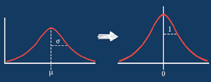
Understanding Standardization

We have standardization as a remedy to the issue that has emerged. It assists in resolving this by:

• Down converting the values to a universal scale, generally ranging from -1 to +1.
• As well as maintaining the range between the values.

We can also represent it through the mathematical formula i.e.,

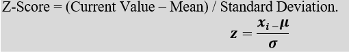
We are substituting the Z-Score for each and every input value using this formula. As a result, we obtain numbers that maintain the range from -1 to +1.

The following are the implications of standardization:

• Conversion of Mean() to 0
• Conversion of Standard Deviation() to 1

Implementation of Code

Here we will do standardization without any special function.

We are going to do the following work:

• Computing the Z-Scores
• Comparison of Original values and standardized values
• Comparison of the Range of both using Scatter Plots

# Importing Libraries
import matplotlib
import matplotlib.pyplot as plt


# We are just using 10 values for our dataset
#For our Dataset, we are going to use 10 random values


# keep in mind that dataset_zero will be constant and it ranges from 1 to 10.
# But, dataset_one will be scaled down as it ranges from 1 to 95000.


global  dataset_zero, dataset_one
dataset_zero = [1,2,3,4,5,6,7,8,9,10]
dataset_one = [35464,50826,7,94142,541,6859,5,789,99,1]




n = len(dataset_one)
mean_ans = 0
ans = 0
j = 0


# Computing Summation
for i in dataset_one:
    j = j + i
    k = i*i
    ans = ans + k


print('n : ', n)
print("Summation (x) : ", j)
print("Summation (x^2) : ", ans)

Output:

# Computing Standard Deviation
part_1_ = ans/n
part_2_ = mean_ans*mean_ans
standard_deviation_ = part_1_ - part_2_
print("Standard Deviation : ", standard_deviation_)

Output:

Standard Deviation :  2550332939.0

# Computing Mean
mean = j/n
mean

Output:

37746.6

# Computing  the Z-Score for each value of dataset_one
final_z_score_ = []
print("Computing Z-Score of Each Value in dataset_one")


for i in dataset_one:
    z_score = (i-mean)/standard_deviation_
    final_z_score_.append("{:.20f}".format(z_score))

Output:

Computing Z-Score of Each Value in dataset_one

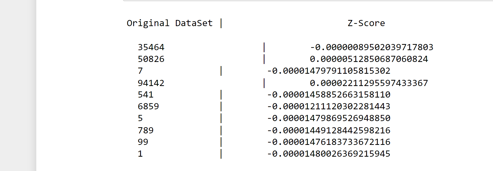
# Comparison of the Values of the Original Dataset and Scaled Down Dataset
print("\nOriginal DataSet |          Z-Score ")
print()
for i in range(len(dataset_one)):
    print(" ", dataset_one[i], "         |   ", final_z_score_[i])

Output:

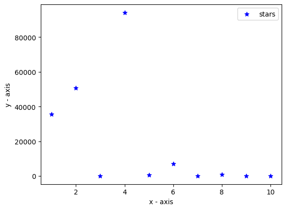
# Graph  of the Original Values
plt.scatter(dataset_zero, dataset_one, label="stars",
            color="blue", marker="*", s=40)
plt.xlabel('x - axis')
plt.ylabel('y - axis')
plt.legend()
plt.show()

Output:

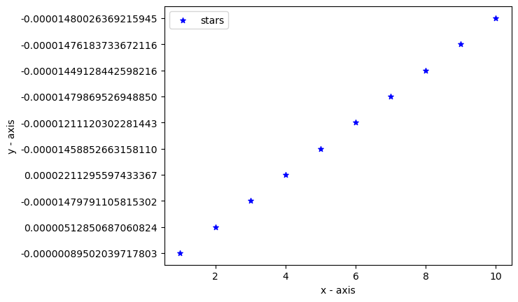
#  Graph of the Standardized Values


plt.scatter(dataset_zero, final_z_score_, label="stars",
            color="blue", marker="*", s=30)
plt.xlabel('x - axis')
plt.ylabel('y - axis')
plt.legend()
plt.show()

Output:

In the above section, we have done the standardization through manual computing with the help of the standardization formula, Although the Scikit-learn package provides the StandardScaler function.

Working On Dataset

So, now we are going to do standardization on a kaggle dataset.

Dataset:Social_Network_Ads.csv

Link of Dataset:https://www.kaggle.com/code/jayoza198/standardization-in-machine-learning/data

#Importing the required Libraries
import numpy as np
import pandas as pd
import matplotlib.pyplot as plt
import seaborn as sns




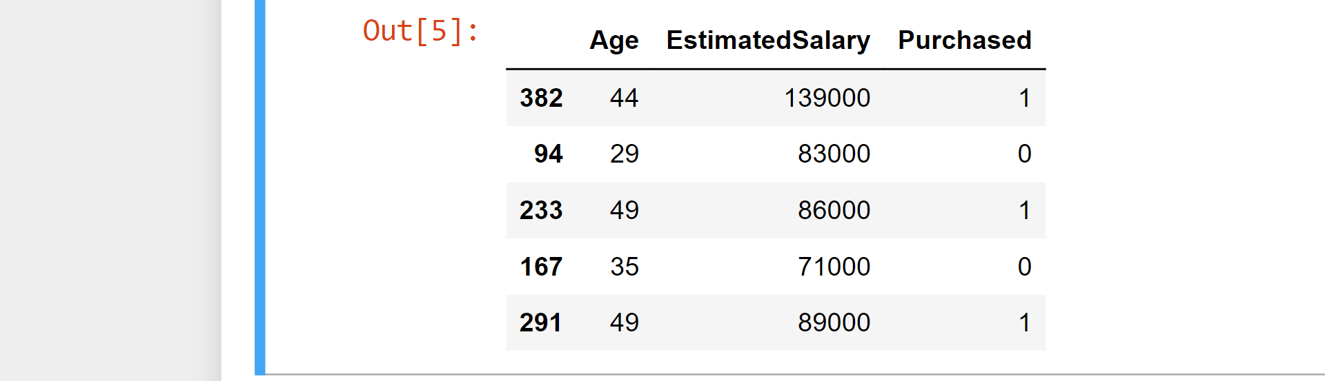
# Loading the Dataset
af = pd.read_csv('Social_Network_Ads.csv')


af=af.iloc[:,2:]


af.sample(5)

Output:

# Train-Test Split
#Splitting the dataset into two parts: Train-Set and Testing-Set


from sklearn.model_selection import train_test_split
X_train, X_test, y_train, y_test = train_test_split(af.drop('Purchased', axis=1),
                                                    af['Purchased'],
                                                    test_size=0.3,
                                                    random_state=0)


X_train.shape, X_test.shape

Output:

((280, 2), (120, 2))

#StandardScaler
from sklearn.preprocessing import StandardScaler


scaler = StandardScaler()


#Fitting the scaler to the train set
scaler.fit(X_train)




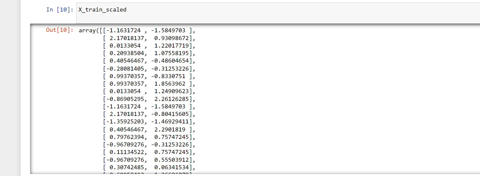
X_train_scaled = scaler.transform(X_train)
X_test_scaled = scaler.transform(X_test)


scaler.mean_

Output:

array([3.78642857e+01, 6.98071429e+04])

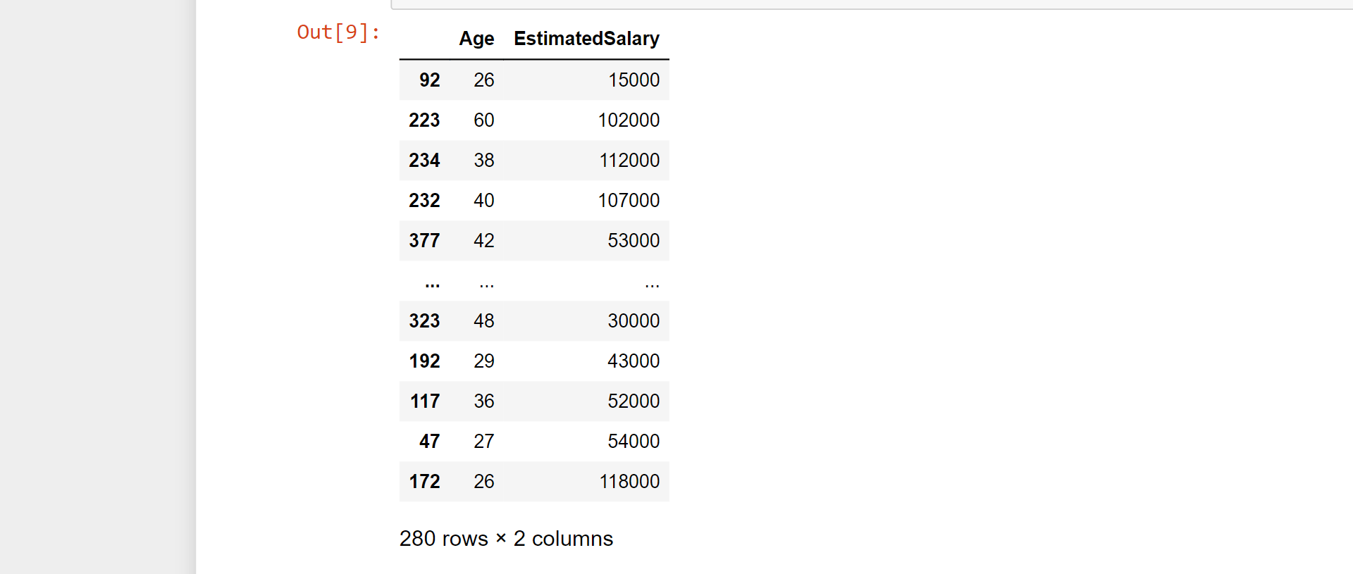
In [9]:

X_train

Output:

X_train_scaled

Output:

X_train_scaled = pd.DataFrame(X_train_scaled, columns=X_train.columns)
X_test_scaled = pd.DataFrame(X_test_scaled, columns=X_test.columns)


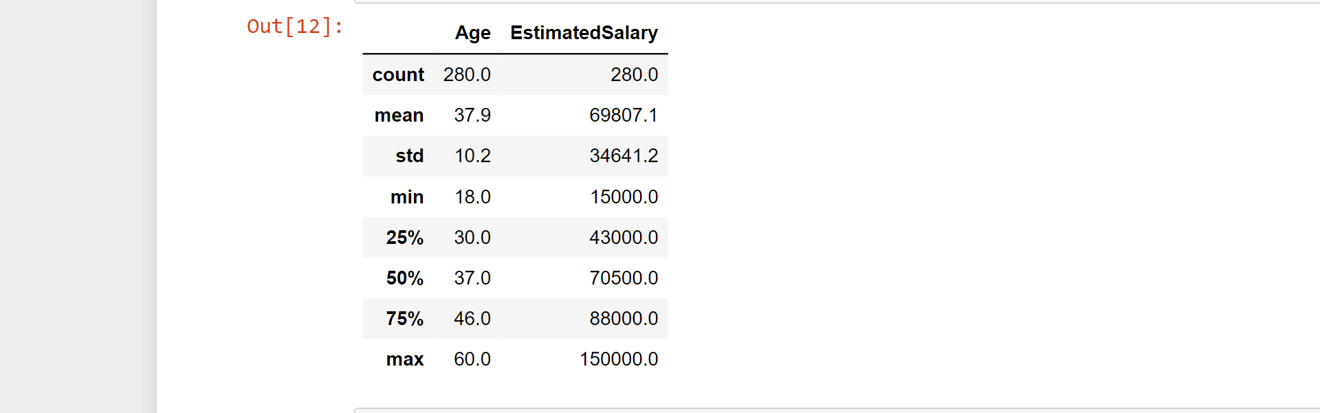
np.round(X_train.describe(), 1)

Output:

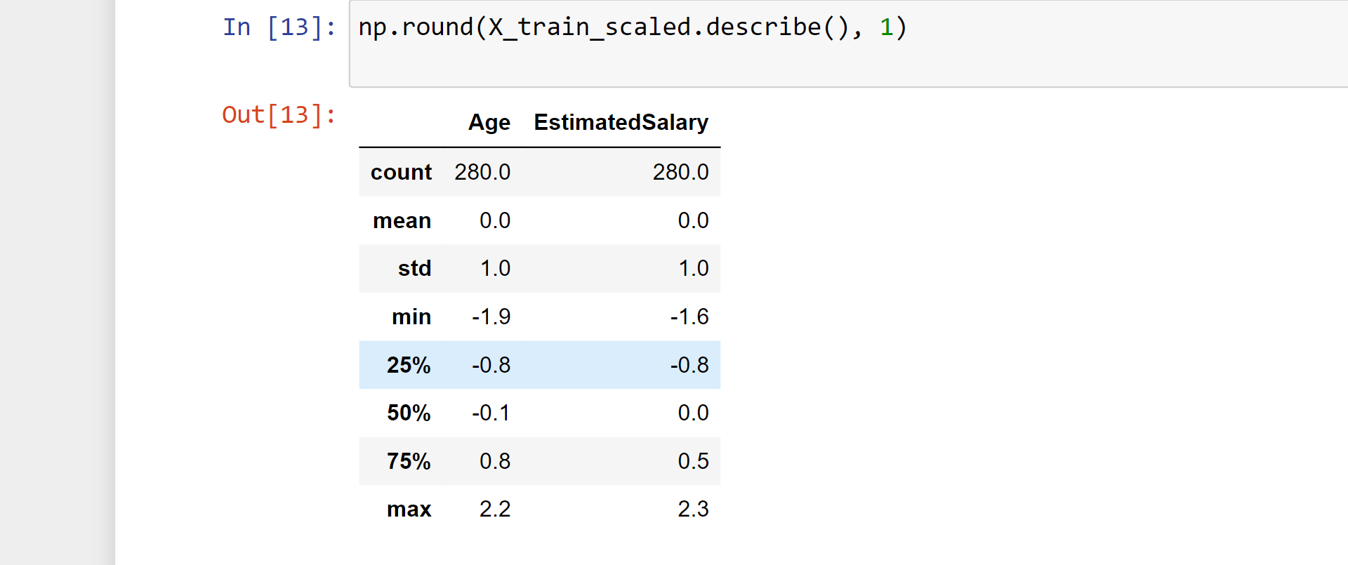
np.round(X_train_scaled.describe(), 1)

Output:

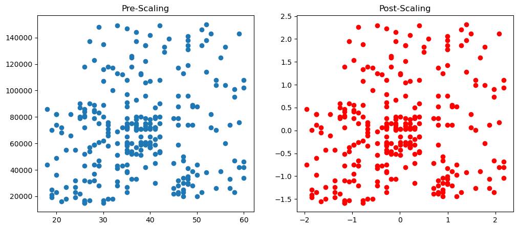
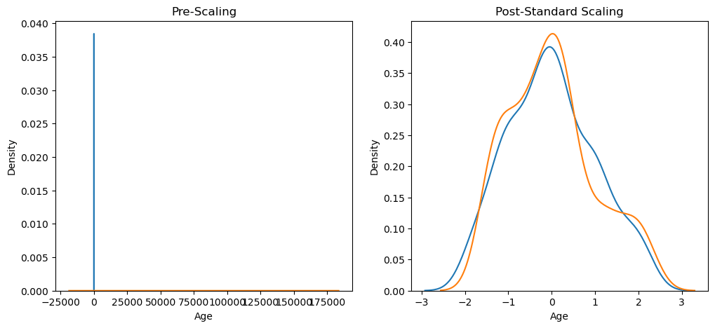
Effects of Standard Scaling

Standardization sometimes causes changes in the distribution, so here we will look in the changes caused by standard scaling.

fig, (ax1, ax2) = plt.subplots(ncols=2, figsize=(12, 5))


ax1.scatter(X_train['Age'], X_train['EstimatedSalary'])
ax1.set_title("Pre-Scaling")
ax2.scatter(X_train_scaled['Age'], X_train_scaled['EstimatedSalary'],color='red')
ax2.set_title("Post-Scaling")
plt.show()

Output:

fig, (ax1, ax2) = plt.subplots(ncols=2, figsize=(12, 5))


# before scaling
ax1.set_title('Pre-Scaling')
sns.kdeplot(X_train['Age'], ax=ax1)
sns.kdeplot(X_train['EstimatedSalary'], ax=ax1)


# after scaling
ax2.set_title('Post-Standard Scaling')
sns.kdeplot(X_train_scaled['Age'], ax=ax2)
sns.kdeplot(X_train_scaled['EstimatedSalary'], ax=ax2)
plt.show()

Output:

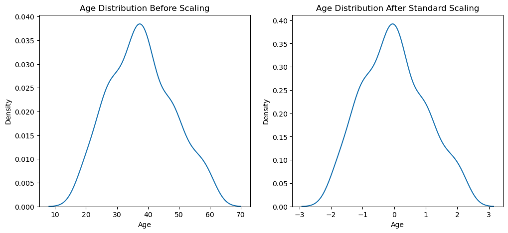
Distribution Comparison

Here, We will compare the distribution that is caused by the standard scaling.

fig, (ax1, ax2) = plt.subplots(ncols=2, figsize=(12, 5))


# Pre-Scaling
ax1.set_title('Age Distribution Before Scaling')
sns.kdeplot(X_train['Age'], ax=ax1)


# Post-Scaling
ax2.set_title('Age Distribution After Standard Scaling')
sns.kdeplot(X_train_scaled['Age'], ax=ax2)
plt.show()

Output:

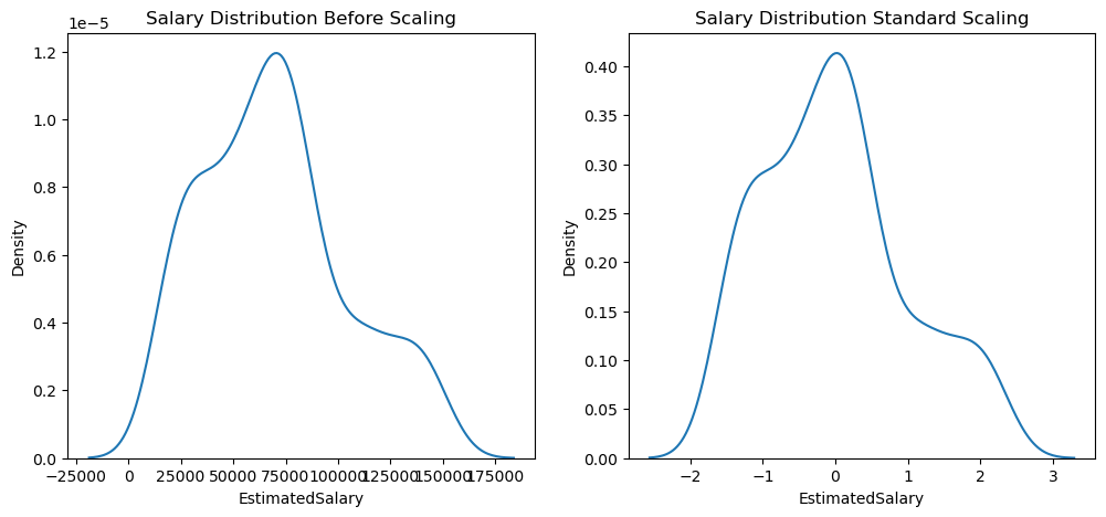
fig, (ax1, ax2) = plt.subplots(ncols=2, figsize=(12, 5))


# Pre-scaling
ax1.set_title('Salary Distribution Before Scaling')
sns.kdeplot(X_train['EstimatedSalary'], ax=ax1)


# Post-scaling
ax2.set_title('Salary Distribution Standard Scaling')
sns.kdeplot(X_train_scaled['EstimatedSalary'], ax=ax2)
plt.show()

Output:

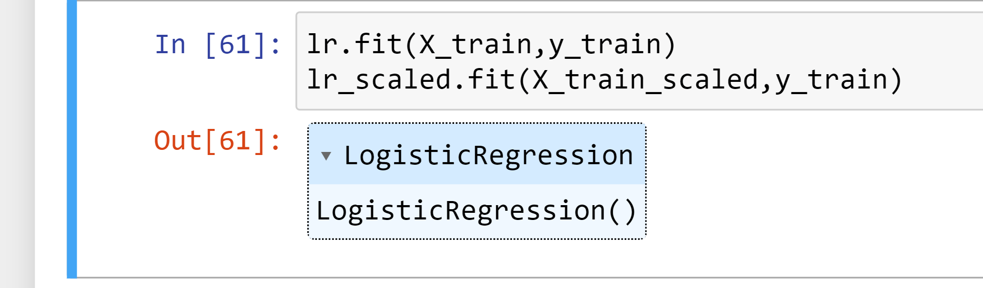
Importance of Standardization

Now, we will test the standardization with the logistic regression and decision tree algorithm.

from sklearn.linear_model import LogisticRegression

from sklearn.linear_model import LogisticRegression
lr = LogisticRegression()
lr_scaled = LogisticRegression()
lr.fit(X_train,y_train)
lr_scaled.fit(X_train_scaled,y_train)

Output:

y_pred = lr.predict(X_test)
y_pred_scaled = lr_scaled.predict(X_test_scaled)


from sklearn.metrics import accuracy_score


print("Actual",accuracy_score(y_test,y_pred))
print("Scaled",accuracy_score(y_test,y_pred_scaled))

Output:

Actual 0.6583333333333333
Scaled 0.8666666666666667
The actual prediction and scaled prediction are notsimilar.

from sklearn.tree import DecisionTreeClassifier
dt = DecisionTreeClassifier()
dt_scaled = DecisionTreeClassifier()
dt.fit(X_train,y_train)
dt_scaled.fit(X_train_scaled,y_train)

Output:

y_pred = dt.predict(X_test)
y_pred_scaled = dt_scaled.predict(X_test_scaled)
print("Actual",accuracy_score(y_test,y_pred))
print("Scaled",accuracy_score(y_test,y_pred_scaled))

Output:

Actual 0.875
Scaled 0.8666666666666667


The actual prediction and scaled prediction are quite similar.