Machine Learning for Audio Classification

Pitch detection, speech recognition, musical instrument understanding, and music creation are all possible uses for machine learning. For our situation, audio categorization will be done using machine learning.

When assessing the surroundings using photographs, machine learning has produced excellent results. Audio categorization hasn't properly tapped into this sector, though.

This is because, unlike a camera, sound may provide us with a nondirectional perspective. Lighting has no impact on the sound. This indicates that regardless of the time of day or night, you may hear the sound in the same way. Instead, we might use machine learning by converting sound waves into audio and spectrograms (visual representations of frequencies).

Pitch recognition and music creation may both benefit from audio machine learning.

When a computer must decide if an audio file is a speech or music, this is a prime illustration of an audio categorization issue.

Difference between Audio and Sound

The things you hear are sounds. The sound wave is actually a vibration that is being transmitted. Frequencies, speed, loudness, and direction are particular aspects of sound.

Only frequency and amplitude are the crucial characteristics in this domain, where machine learning is mostly used.

Sinusoidal waves are a common simplification of sound waves. A sinusoidal wave demonstrates how a variable's amplitude fluctuates over time. Sound is captured with a mic and converted to an electronic representation.

Sound is represented electronically through audio. Sounds having frequencies between 20Hz and 20kHz that can be heard by humans.

Humans cannot hear frequencies below 20Hz or over 20KHz because they are either too low or too high.

Spectrogram

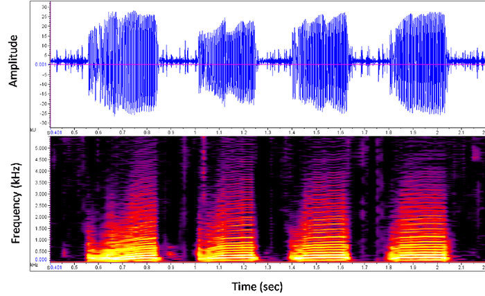
The visual depiction of all frequencies throughout time is a spectrogram.

The time scale is on the X-axis, while the frequency in hertz is on the Y-axis. The size or amplitude is shown by the hue. A spectrogram's color is measured in decibels and is either brighter or higher (unit of measure).

A waveform can be transformed into a spectrogram. This is comparable to a picture, technically. Researchers have discovered computer vision methods may be successfully used on spectrograms.

This implies that the techniques used to categorize images may also be used to evaluate the sound. A machine learning model may extract the dominant audio per time frame in a waveform by spotting patterns in the spectrogram.

We won't be looking for patterns using a spectrogram, though. To do this, we'll use a library called Librosa.

Now we will implement it.

Exploration Data Analysis

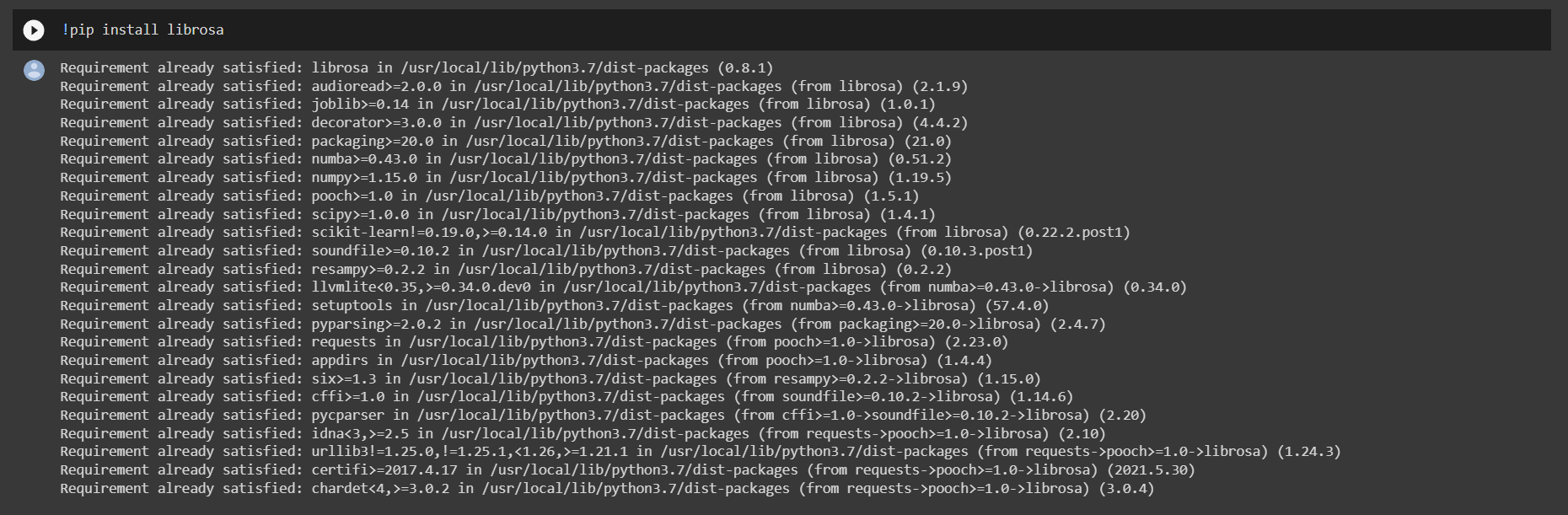
Installing Librosa is required for this, and the following command will be used:

!pip install librosa

Output:

Then We need to import all the required Libraries:

import pandas as pd
import os
import librosa
import librosa.display
import numpy as np
import IPython.display as ipd
from tqdm import tqdm
import matplotlib.pyplot as plt
%matplotlib inline

Loading the Dataset

Now we have to import our external Kaggle data into Google Colab. For that, we need to follow the underlying steps:

Step 1:Download your Kaggle API token by visiting your Kaggle account. It may be found under the API section. When you select the Create New API Token button, a kaggle.json file will be generated and downloaded to your computer.

Step 2:You have to upload the kaggle.json file to your colab project that you just downloaded.

Step 3:The current working directory should be added to the KAGGLE_CONFIG_DIR path as shown:

import os
os.environ['KAGGLE_CONFIG_DIR'] = "/content"

Note: Simply type !pwd in the terminal to access your current working directory.

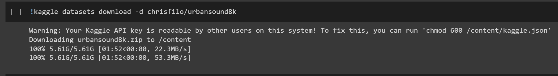
Step 4:To download datasets, use the following Kaggle API command:

!kaggle datasets download -d chrisfilo/urbansound8k

Output:

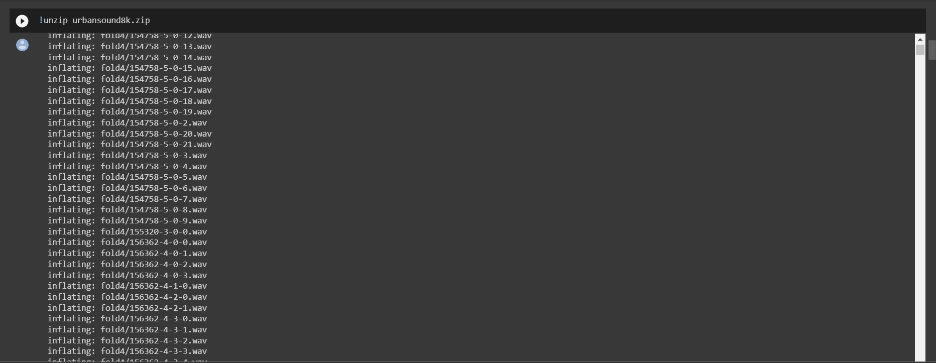
As now you have downloaded the dataset, you have to unzip the downloaded dataset, and for that, you have to follow the underlying command.

!unzip urbansound8k.zip

Output:

Note: You can download the kaggle dataset from the following link.

https://www.kaggle.com/datasets/chrisfilo/urbansound8k/download?datasetVersionNumber=1

Experimenting

We need to do a little bit of analysis on simple audio, so here we will do an analysis of an audio file of children playing(100263-2-0-121.wav) from the dataset.

file_name='fold5/100263-2-0-121.wav'


audio_data, sampling_rate = librosa.load(file_name)
librosa.display.waveplot(audio_data,sr=sampling_rate)
ipd.Audio(file_name)

Output:

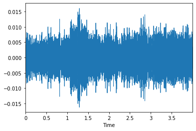
Both the audio data and sampling rate are provided by Librosa. Let's look at the outcomes for a single example audio file:

audio_data

Output:

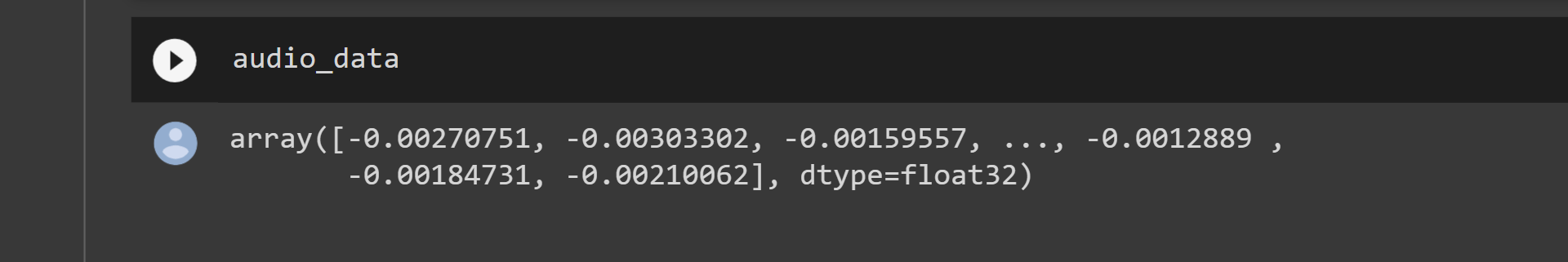
There is only one signal in mono. As a consequence, our audio data findings demonstrate that Librosa transformed the audio into single-dimensional integers.

We would have had two signals and a 2D array if it had been stereo. Stereo sound is typically favored in audio. However, we won't be using stereo signals in our article.

These signals are condensed by Librosa into mono for simpler processing. It provides us with a feeling of orientation, perspective, and space.

sampling_rate

Output:

22050

Note: Librosa provides us with a sample rate of 22050 by default.

Now we will employ Pandas library for reading CSV files:

audio_dataset_path='/content/'
metadata=pd.read_csv('UrbanSound8K.csv')
metadata.head()

Output:

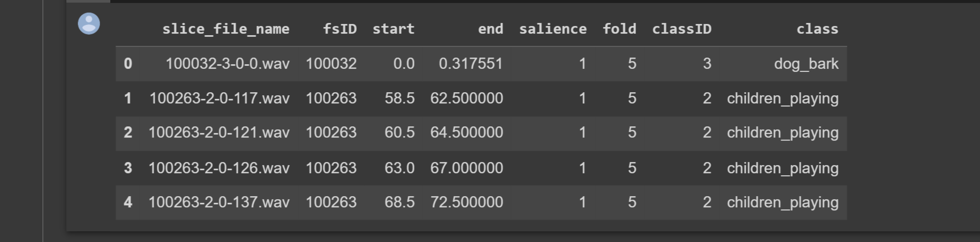
We can observe that the audio files are all kept in the .wav file type. Additionally, they are arranged into the appropriate file classifications.

There should be no imbalance in our dataset. We use the following command to quickly verify that it isn't:

metadata['class'].value_counts()

Output:

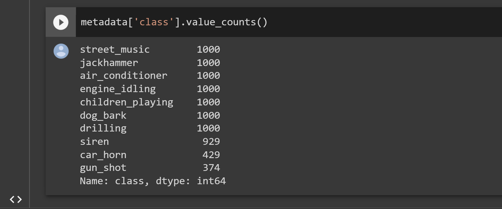
The findings indicate that the majority of the dataset's classes are balanced. As a result, using this dataset would be wise.

We have concluded that this data is in its raw format now that EDA is complete. To extract useful characteristics from this data, preprocessing is required.

Instead of using the data in its original form for training, we will employ these derived characteristics.

Data Processing

We will employ the Mel-Frequency Cepstral Coefficients (MFCC) technique to extract the features.

The frequency distribution across the window size is summarised by the MFCC method. This makes it possible to analyze the given sound's frequency and temporal properties. We may use it to find characteristics for categorization.

mfccs = librosa.feature.mfcc(y=audio_data, sr=sampling_rate, n_mfcc=40)

The number of MFCCs to return is indicated by the n mfcc argument. For our scenario, we went with 40. Any value that you desire can be selected.

mfccs

Output:

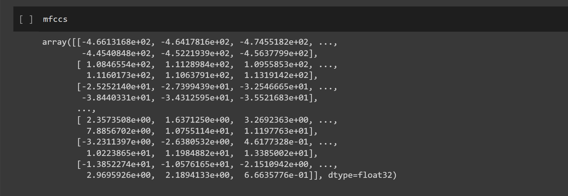
Based on the frequency and timing properties of the audio clip, these patterns were derived from it.

def features_extractor(file):
    audio, sample_rate = librosa.load(file_name, res_type='kaiser_fast')
    mfccs_features = librosa.feature.mfcc(y=audio, sr=sample_rate, n_mfcc=40)
    mfccs_scaled_features = np.mean(mfccs_features.T,axis=0)
   
    return mfccs_scaled_features

We establish a list to contain all the collected features after extracting the features from each audio file in the dataset.

After that, we repeatedly go over each audio file and use the Mel-Frequency Cepstral Coefficients to extract features.

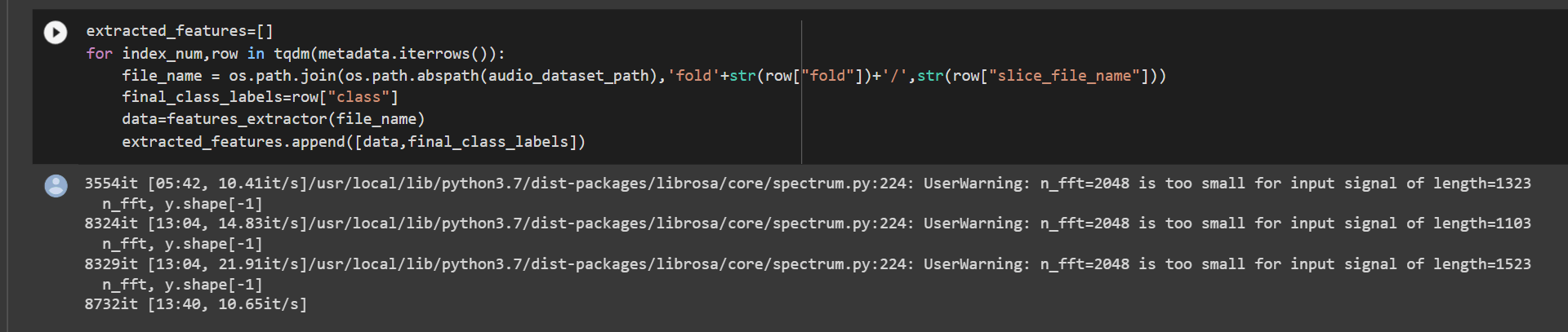
extracted_features=[]
for index_num,row in tqdm(metadata.iterrows()):
    file_name = os.path.join(os.path.abspath(audio_dataset_path),'fold'+str(row["fold"])+'/',str(row["slice_file_name"]))
    final_class_labels=row["class"]
    data=features_extractor(file_name)
    extracted_features.append([data,final_class_labels])

Output:

Let's use the Pandas package to turn the complete list into a data frame. As a consequence, the findings are transformed into tables for easier analysis.

extracted_features_df=pd.DataFrame(extracted_features,columns=['feature','class'])
extracted_features_df.head(10)

Output:

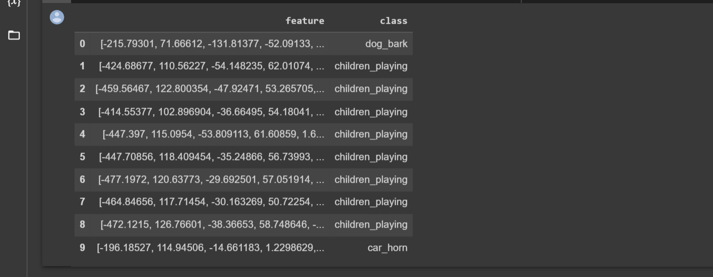
The extracted characteristics and the classes for each are displayed in the results above.

The dataset is divided into independent and dependent datasets, x and y, using the following command.

X=np.array(extracted_features_df['feature'].tolist())
y=np.array(extracted_features_df['class'].tolist())
X.shape

Output:

(8732, 40)

y

Output:

array(['dog_bark', 'children_playing', 'children_playing', ...,
       'car_horn', 'car_horn', 'car_horn'], dtype='<U16')

y.shape

Output:

(8732,)

Then, we import the categorical and LabelEncoder TensorFlow and Sklearn algorithms.

from tensorflow.keras.utils import to_categorical
from sklearn.preprocessing import LabelEncoder
labelencoder=LabelEncoder()
y=to_categorical(labelencoder.fit_transform(y))


y

Output:

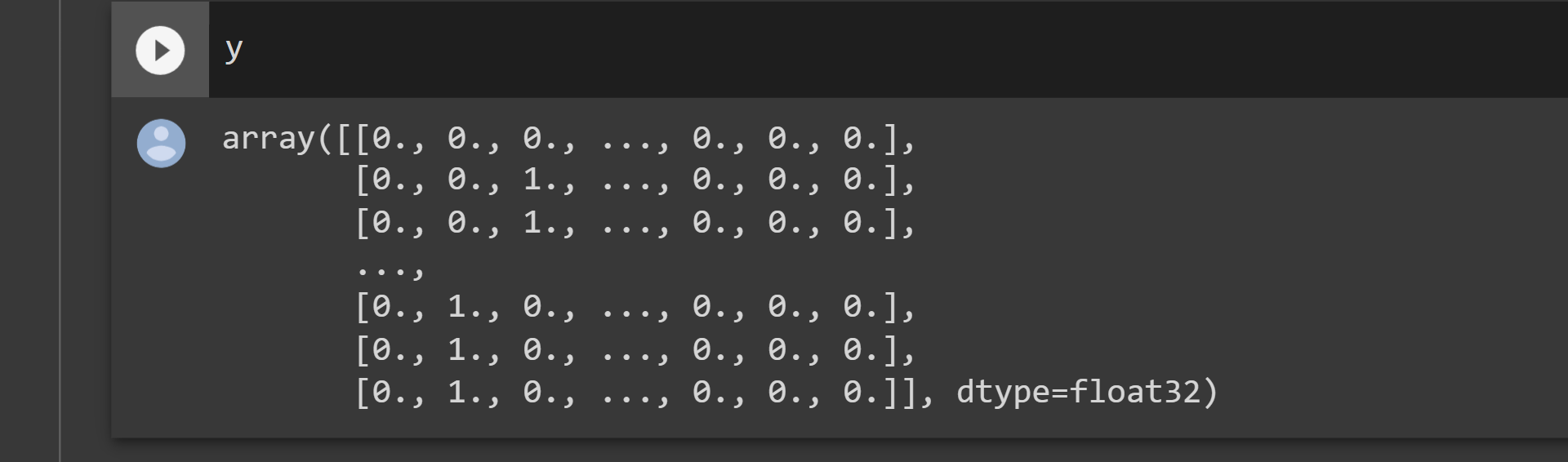
y.shape

Output:

(8732, 10)

Dividing our dataset into training and test sets with sklearn's train test split technique.

from sklearn.model_selection import train_test_split

X_train,X_test,y_train,y_test=train_test_split(X,y,test_size=0.2,random_state=0)

Model Creation

We'll use TensorFlow to build a model.

#Imporing tensorflow in the notebook
import tensorflow as tf
print(tf.__version__)

Output:

2.6.0

from tensorflow.keras.models import Sequential
from tensorflow.keras.layers import Dense,Dropout,Activation,Flatten
from tensorflow.keras.optimizers import Adam
from sklearn import metrics


num_labels=y.shape

We'll stack our layers in order. It is a multi-class classification issue, hence the final layer will feature a softmax activation layer.

model=Sequential()
#first layer
model.add(Dense(100,input_shape=(40,)))
model.add(Activation('relu'))
model.add(Dropout(0.5))
#second layer
model.add(Dense(200))
model.add(Activation('relu'))
model.add(Dropout(0.5))
#third layer
model.add(Dense(100))
model.add(Activation('relu'))
model.add(Dropout(0.5))


#final layer
model.add(Dense(num_labels))
model.add(Activation('softmax'))

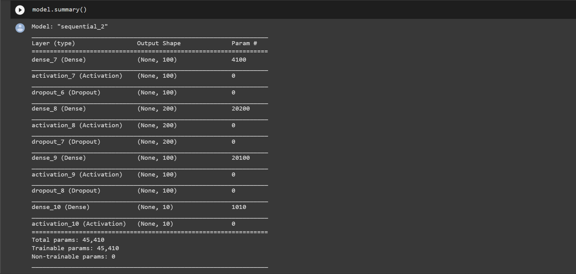
We can also look at the summary of the model

model.summary()

Output:

model.compile(loss='categorical_crossentropy',metrics=['accuracy'],optimizer='adam')

Our model can now be trained. The precision rises as the number of epochs grow. In our instance, we just used 200 epochs to train the model.

From tensorflow.keras.callbacks import ModelCheckpoint
from datetime import datetime


num_epochs = 200
num_batch_size = 32


checkpointer = ModelCheckpoint(filepath='saved_models/audio_classification.hdf5',
                               verbose=1, save_best_only=True)
start = datetime.now()


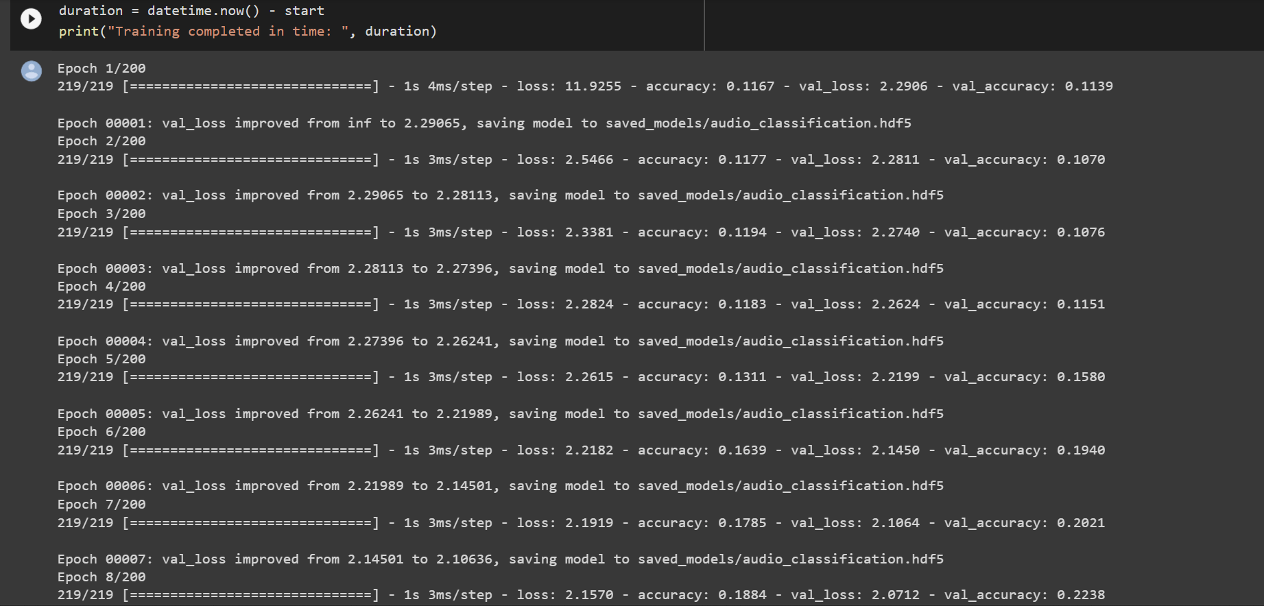
model.fit(X_train, y_train, batch_size=num_batch_size, epochs=num_epochs, validation_data=(X_test, y_test), callbacks=[checkpointer], verbose=1)




duration = datetime.now() - start
print("Training completed in time: ", duration)

Output:

Running the following code yields the validation accuracy:

test_accuracy=model.evaluate(X_test,y_test,verbose=0)
print(test_accuracy[1])

Output:

0.7870635390281677

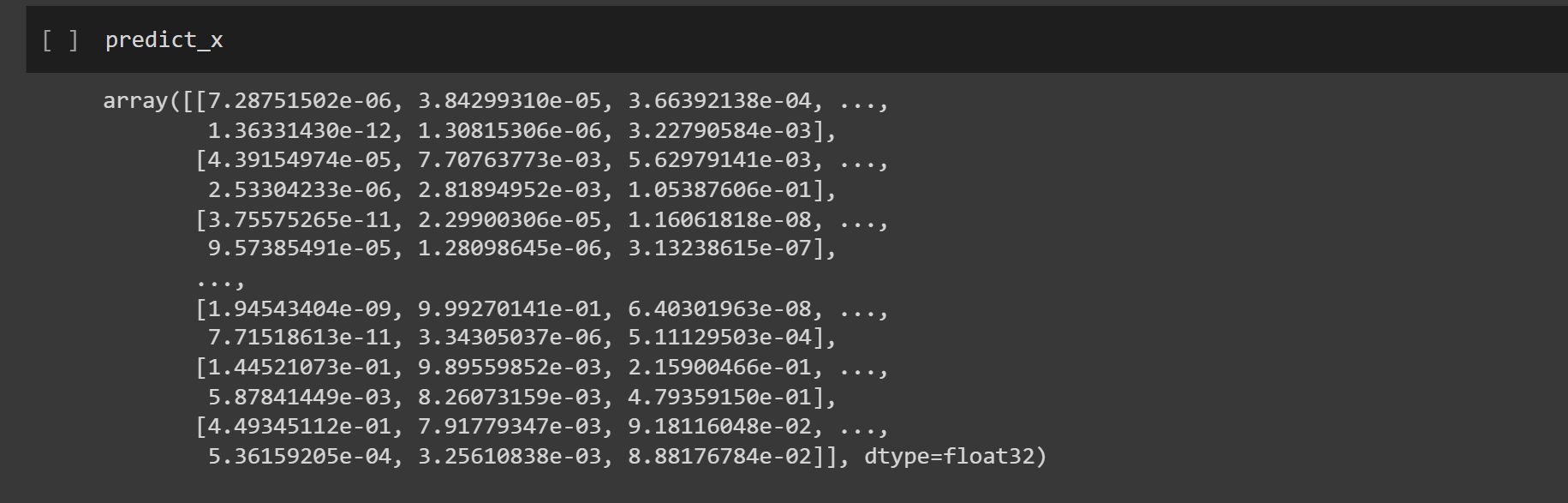
predict_x=model.predict(X_test)
classes_x=np.argmax(predict_x,axis=1)


predict_x

Output:

classes_x

Output:

array([5, 3, 4, ..., 1, 9, 0])

Testing the Model

The three actions listed below will be carried out in this section:

• Preparing the audio test data. It entails utilizing the MFCC method to extract the characteristics.
• Determining its class with the aid of the model we developed.
• To obtain our class label, invert and convert the expected label.

From our dataset, we randomly select the dog-barking audio file 103076-3-0-0.wav to utilize for testing. Now we have to go over the procedures we used to preprocess audio data once again.

The predicted label name is then obtained by doing a prediction of the class to which it belongs, followed by using the inverse transform function from sci-kit-learn.

filename="fold8/103076-3-0-0.wav"
audio, sample_rate = librosa.load(filename, res_type='kaiser_fast')
mfccs_features = librosa.feature.mfcc(y=audio, sr=sample_rate, n_mfcc=40)
mfccs_scaled_features = np.mean(mfccs_features.T,axis=0)


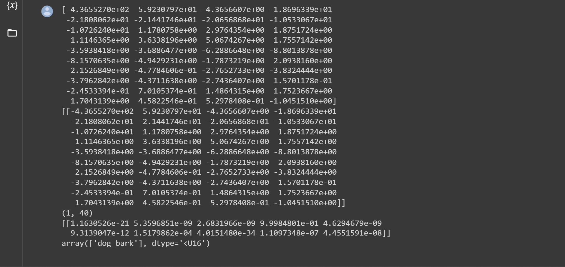
print(mfccs_scaled_features)
mfccs_scaled_features=mfccs_scaled_features.reshape(1,-1)
print(mfccs_scaled_features)
print(mfccs_scaled_features.shape)
predicted_label=model.predict(mfccs_scaled_features)
print(predicted_label)
classes_x=np.argmax(predicted_label,axis=1)
prediction_class = labelencoder.inverse_transform(classes_x)
prediction_class

Output:

Summing Up

There are several difficulties in audio signal processing for developers. However, it is much simpler to grasp if you use libraries like Librosa.

The Librosa library is not required for this activity. If you already have the waveform, you may turn it into a spectrogram and classify the data with a Convolution Neural Network (CNN).