Linear Regression in Machine learning
Introduction to Linear Regression
Linear regression is the most important statistical algorithm in machine learning to learn the correlation between a dependent variable and one or more independent features. So, we can say that the linear relation between two variables can be stated as the change (increase/decrease) in the value of the dependent variable in accordance to the change in the value of independent variables.
Mathematically it can be written as;
Y=mX+C
Where Y is a dependent variable called as responses, m is the regression coefficient, X is the independent variable called as predictors, and C is the constant. The value of C is called as intercept shows the point where the line of regression crosses the Y-axis, and m calculates the slope of the evaluated regression line.
A linear relationship is of two types:
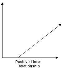
1. Positive Linear Relationship: If both dependent variable as well as independent variables increases, then a linear relationship is known as Positive Linear Relationship. It can be more clearly understood by the image given below:
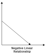
2. Negative Linear Relationship: With the increase in the independent variable, if the dependent variable decreases, then that linear relationship is termed as Negative Linear Relationship. It can be more clearly understood by the image given below:
Types of Linear Regression:
1)Simple Linear Regression:
It is one of the widely used regression technique. It is easy to interpret the results. It is the basic type of linear regression and forecasts the result based on a single feature. It assumes that two of its variable are linearly interconnected.
To deploy the simple linear regression model, we will undergo some of the following steps:
Step 1:
The first step is data pre-processing, as we did earlier. In this, we will first import the libraries to get the essential tools which help us in building our model and the dataset.
import numpy as np
import pandas as pd
import matplotlib.pyplot as plt
dataset= pd.read_csv(' Salary_Data.csv')
This is the dataset which we get from the above code:
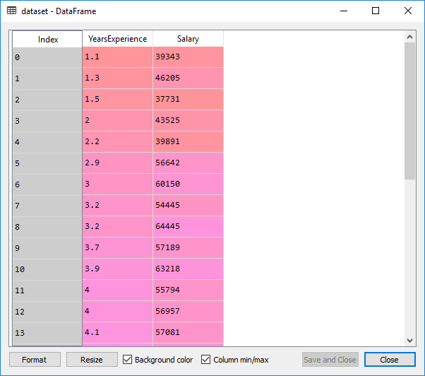
The dataset contains two columns; the years of experience and salary, which is an information of employees working in the company. We will train our model that will learn the correlation between no. of years of experience each employee has and their salary.
After that, we will split the dataset into the training set and test set.
X= dataset.iloc [:,:-1].values
Y= dataset.iloc [: ,1].values
From the above-given code, we get the following output on clicking X or Y in variable explorer:
For X:
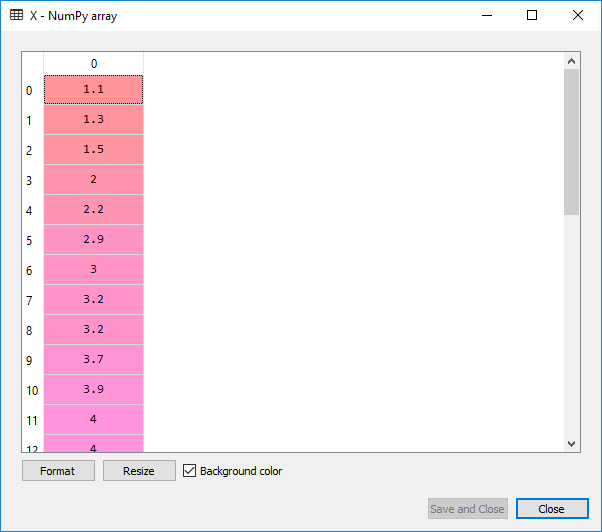
Here X is the matrix features or the independent variables, and Y is the vector of the dependent variables. We will not perform feature scaling as the library will do itself.
Now we will split the dataset into a training set and the test set. The random state parameter is set to 0 so that we can get the same results as some random factors are present in the algorithm.
from sklearn. model_selection import train_test_split
X_train, X_test, Y_train, Y_test=train_test_split(X,Y,test_size=1/3,random_state=0)
On executing the above two lines, we will get the following output when we click on X_train in variable explorer:
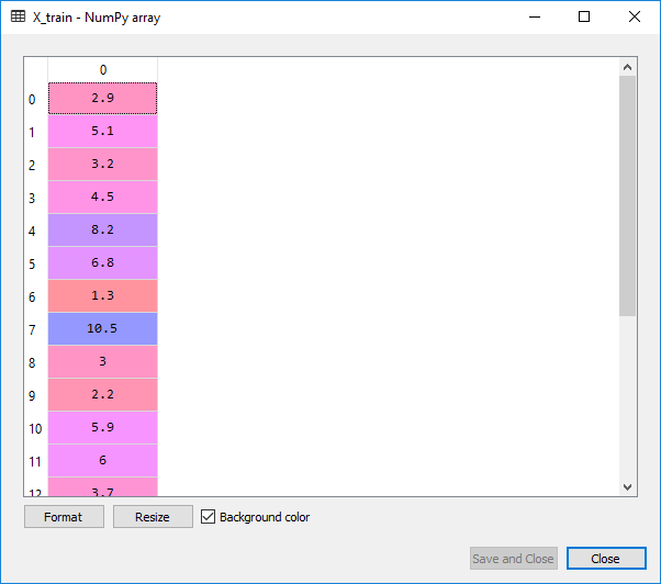
Here X_train and Y_train form a training set, whereas X_test and Y_test form a test set. The model will learn from the correlation between X_train and Y_train of the training set so that their power of prediction will be tested on a test set.
Step 2:
In this step, we will first fit the simple linear regression algorithm to the training set, and for that, we first need to import a library linear_model from the scikit learn. Then we will create an object of linear regression class which will be the simple linear regressor.
from sklearn.linear_model import LinearRegression
regressor =LinearRegression()
regressor.fit(X_train, Y_train)
Output:
LinearRegression(copy_X=True, fit_intercept=True, n_jobs=None, normalize=False)
Now that the simple linear regressor has learned the relations between the no of user’s experience and their salary to learn how they predict the salary based on the experience.
We will create a vector of predicted values, and it will contain the prediction of the test set salaries, and we will see all these salaries in the single vector called Y_pred which is a vector prediction of the dependent variable.
Y_pred=regressor.predict(X_test)
Upon execution of this code, a variable called Y_pred will get built in the variable explorer pane, containing the predicted salary of 10 observation in the test case. You can check it by clicking on the Y_pred.
Output:
To compute the difference between the actual salary and the predicted you can do by comparing the Y_pred to Y_test, also you can see how best your simple linear model is in making the predictions.
In the last step, we will visualize the training set as well as the test set. And for that, we will plot the observation points and the simple linear regression to see how there are linear dependency and the prediction of a simple linear model to the real observations. To plot the graph, we will import the matplot library
Visualization of the training set:
plt.scatter(X_train,Y_train, color='red')
plt.plot(X_train,regressor.predict(X_train),color='blue')
plt.title('Salary vs Experienced(Training set)')
plt.xlabel('Years of experience')
plt.ylabel('Salary')
plt.show()
Output:
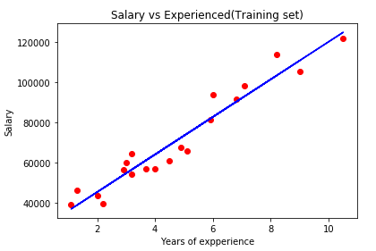
From the above-presented image, the real values of the employees are the red dots, and the predicted values (predicted salary) are on the blue simple regression line. This shows a clear linear dependency between the salary and years of experience.
Since the regression line is approaching quite well to all the observation points, we can fit a good simple linear regression model that gives a good prediction. It can be seen from the output image that the real salary is much close to the predicted salary.
Now we will see how the simple linear regression model works for the new observations (test set), as the model is not trained on the test set. We will now plot for the test case.
Visualization of Test set:
plt.scatter(X_test,Y_test, color='red')
plt.plot(X_train,regressor.predict(X_train),color='blue')
plt.title('Salary vs Experienced(Training set)')
plt.xlabel('Years of expperience')
plt.ylabel('Salary')
plt.show()
Output:
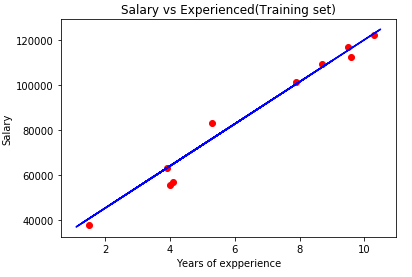
Here the red points are the observation points of the test set and blue line is simple linear regression line that contains the predicted values. The prediction made is quite good, as we have made good simple linear regression model which is perfectly able to predict the observations.
2) Multiple Linear Regression
Multiple linear regression is an enhancement of simple linear regression. The prediction is made using two or more features.
Any dataset with n no. of observations, p independent variables and y as the response-dependent variable the regression line for p features can be mathematically written as;
F(xi)= m0+m1xi1 +m2xi2+………+mpxip
Where, F(Xi) is the response of the predicted value and m0,m1,m2,..mp is the regression coefficients.
Generally, it adds an error to the data which is called as the residual error and modifies the equation as follows;
F(xi)= m0+m1xi1 +m2xi2+………+mpxip+ei
yi=F(xi)+ei
Some assumptions in Regression model:
- Linearity: It states that the relation between the dependent and independent variables should be linear.
- Homoscedasticity: The term Homoscedasticity states that it should maintain the constant variance.
- Multivariate Normality: It is assumed by Multiple Regression that the residuals are normally distributed.
- Lack of Multicollinearity: In this, it is assumed that there is an either little or no multicollinearity in the data.
Several methods to build a model:
- All in one
- Backward-Elimination
- Forward Selection
- Bi-directional Elimination
- Score Comparison
Backward Elimination:
Step1: The first step in the starting is to select a significance level (SL).
Step2: Now fit the whole model with all the possible predictors.
Step3: Look for the highest P-value. If P>SL, then move to step 4, otherwise the model is ready.
Step4: Eliminate the Predictor.
Step5: Fit the model excluding that variable.
Forward Selection:
Step1: To enter a model, select a significance level (e.g. SL = 0.05).
Step2: Now fit all the simple regression models, and select the one with the lowest P-value.
Step3: Preserve this variable, and fit all the promising models with one predictor added to one’s that we are already having.
Step4: Consider the model which is having the lowest p-value, and if P<SL then, go to step 3, otherwise the model is ready.
A stepwise implementation of the MLR model:
Step1: Data Pre-processing:
- Import Libraries.
- Import Dataset.
- Encode Categorical Data.
- Avoid a Dummy Variable Trap.
- Split Dataset into a Training set and Test set.
Step2: Fit Multi Linear Regression to the Training set.
Step3: Predict the Results of the Test set.
Data Pre-processing:
We will first import the libraries and the dataset, as we did in the previous steps.
#importing the libraries
import numpy as np
import pandas as pd
import matplotlib.pyplot as plt
#importing the dataset using the Pandas library
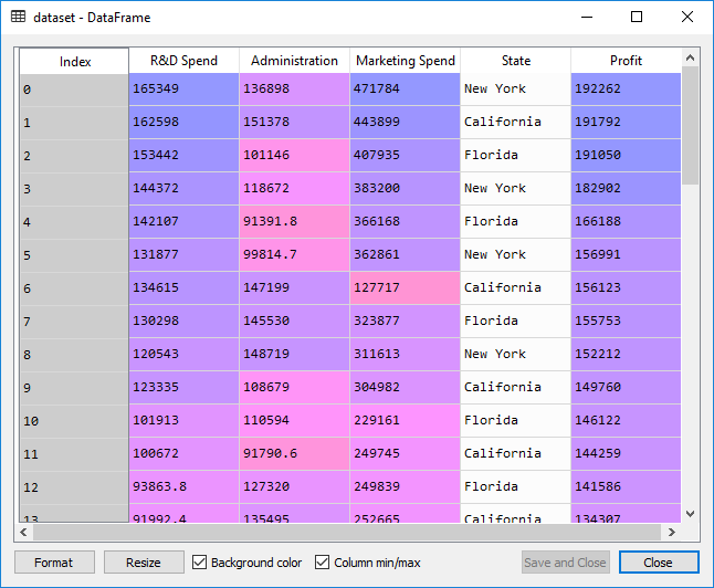
dataset= pd.read_csv('50_Startups.csv')
Here we will use the dataset of 50 start-up companies in the USA. It has the information for a particular financial year; how much money did a company spent on R&D, Administration, Marketing, and how much profit did they earned corresponding to a particular state.
Now we will extract the feature matrix. Here, X is the matrixof the independent variables, and Y is the matrix of the dependent variable vector.
#extracting matrix features
X= dataset.iloc [:,:-1]. values
Y= dataset.iloc [: , 4].values
We cannot have a look at X in the Variable Explorer as the matrix contains different types. So, it cannot select a single type here. But we can see its matrix in IPython console.
Output:
array([[165349.2, 136897.8, 471784.1, 'New York'],
        [162597.7, 151377.59, 443898.53, 'California'],
        [153441.51, 101145.55, 407934.54, 'Florida'],
        [144372.41, 118671.85, 383199.62, 'New York'],
        [142107.34, 91391.77, 366168.42, 'Florida'],
        [131876.9, 99814.71, 362861.36, 'New York'],
        [134615.46, 147198.87, 127716.82, 'California'],
        [130298.13, 145530.06, 323876.68, 'Florida'],
        [120542.52, 148718.95, 311613.29, 'New York'],
        [123334.88, 108679.17, 304981.62, 'California'],
        [101913.08, 110594.11, 229160.95, 'Florida'],
        [100671.96, 91790.61, 249744.55, 'California'],
        [93863.75, 127320.38, 249839.44, 'Florida'],
        [91992.39, 135495.07, 252664.93, 'California'],
        [119943.24, 156547.42, 256512.92, 'Florida'],
        [114523.61, 122616.84, 261776.23, 'New York'],
        [78013.11, 121597.55, 264346.06, 'California'],
        [94657.16, 145077.58, 282574.31, 'New York'],
        [91749.16, 114175.79, 294919.57, 'Florida'],
        [86419.7, 153514.11, 0.0, 'New York'],
        [76253.86, 113867.3, 298664.47, 'California'],
        [78389.47, 153773.43, 299737.29, 'New York'],
        [73994.56, 122782.75, 303319.26, 'Florida'],
        [67532.53, 105751.03, 304768.73, 'Florida'],
        [77044.01, 99281.34, 140574.81, 'New York'],
        [64664.71, 139553.16, 137962.62, 'California'],
        [75328.87, 144135.98, 134050.07, 'Florida'],
        [72107.6, 127864.55, 353183.81, 'New York'],
        [66051.52, 182645.56, 118148.2, 'Florida'],
        [65605.48, 153032.06, 107138.38, 'New York'],
        [61994.48, 115641.28, 91131.24, 'Florida'],
        [61136.38, 152701.92, 88218.23, 'New York'],
        [63408.86, 129219.61, 46085.25, 'California'],
        [55493.95, 103057.49, 214634.81, 'Florida'],
        [46426.07, 157693.92, 210797.67, 'California'],
        [46014.02, 85047.44, 205517.64, 'New York'],
        [28663.76, 127056.21, 201126.82, 'Florida'],
        [44069.95, 51283.14, 197029.42, 'California'],
        [20229.59, 65947.93, 185265.1, 'New York'],
        [38558.51, 82982.09, 174999.3, 'California'],
        [28754.33, 118546.05, 172795.67, 'California'],
        [27892.92, 84710.77, 164470.71, 'Florida'],
        [23640.93, 96189.63, 148001.11, 'California'],
        [15505.73, 127382.3, 35534.17, 'New York'],
        [22177.74, 154806.14, 28334.72, 'California'],
        [1000.23, 124153.04, 1903.93, 'New York'],
        [1315.46, 115816.21, 297114.46, 'Florida'],
        [0.0, 135426.92, 0.0, 'California'],
        [542.05, 51743.15, 0.0, 'New York'],
        [0.0, 116983.8, 45173.06, 'California']], dtype=object)
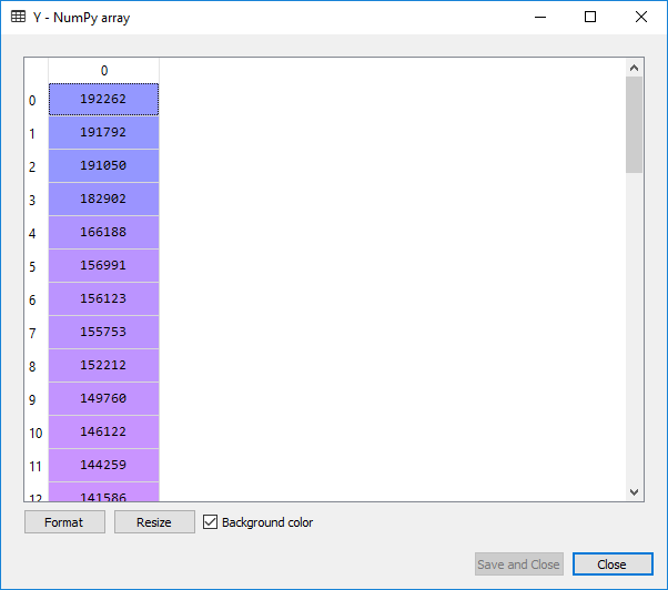
From the above output you can see the four independent variables from R&D spend, Administration spend, Marketing spend as well as the State. To have a look at Y, we can easily open the matrix at Variable Explorer.
On looking at X, you must have noticed the State variable, which is a categorical data and it must be encoded as it contains the text. Because if you keep it like this only, it will cause a problem in machine learning model equations. So, to encode it, we will do exactly the same way as we did in the data pre-processing step. We will use LabelEncoder to encode that particular column in nos. In order to remove the relational order, we will use OneHotEncoder to create the dummy variables.
# Encoding categorical data
from sklearn.preprocessing import LabelEncoder, OneHotEncoder
labelencoder = LabelEncoder()
X[:, 3] = labelencoder.fit_transform(X[:, 3])
onehotencoder = OneHotEncoder(categorical_features = [3])
X = onehotencoder.fit_transform(X).toarray()
Since all our columns are in the same type. The type of independent matrix X is float64 now. We can see it in the image given below:
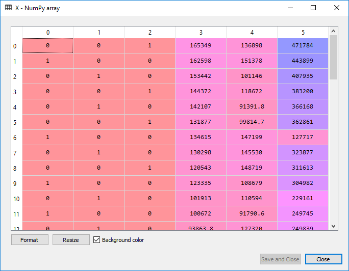
# Avoiding the Dummy Variable Trap
 X = X[:, 1:]
We are removing the first column of X i.e., the column starting at index 0. We only include the columns starting from 1 to end, just to avoid the dummy variable trap.
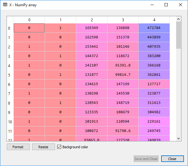
If we look at the image given above, we will see that the first column has been successfully removed which was for California, and for the next time, we would not need to do it manually. It will be taken care of by the python library.
Now we will split the dataset into the training set and the test set. The test set will contain the ten observations, and the training set will have 40 observations.
# Splitting the dataset into the Training set and Test set
from sklearn.model_selection import train_test_split
X_train, X_test, y_train, y_test = train_test_split(X, y, test_size = 0.2, random_state = 0)
Now, will fit the multiple linear regression to the training set as we did in the linear regression model because we are still making a linear regression model but with several independent variables. We are proceeding in the same way as we did in the linear regression model. We will use the fit method to fit the regressor object in the training set.
# Fitting Multiple Linear Regression to the Training set
from sklearn.linear_model import LinearRegression
regressor = LinearRegression()
regressor.fit(X_train, y_train)
Now the next step of this model is the prediction of test set results.
# Predicting the Test set results
y_pred = regressor.predict(X_test)
Upon execution of the above code, we will observe the following predicted value of the test set. We can also compare the real values with the predicted values by clicking at Y_test in variables explorer’s pane.
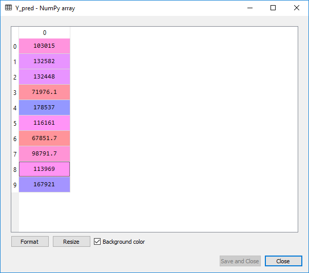
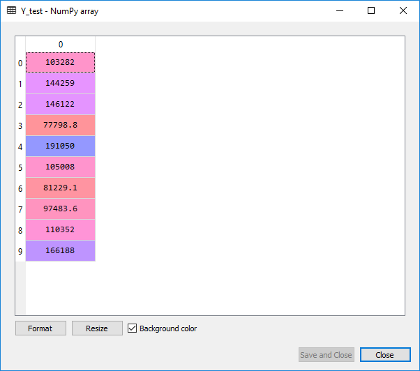
From the above images, we can clearly see that our model did a good job, and it can be seen that there is a multilinear dependency between the independent variables as well as the dependent variables.
Now we will learn some better ways to evaluate our model’s performance. So, do you think we made an optimal model with the given dataset? Because when we built this model, we actually used all the independent variables. But what if among these independent variables some of them are highly statistically significant, means they have a great impact on the dependent variable of profit and some that are not statistically significant at all, which means even if we remove these variables from the model, we will still get some amazing predictions.
The main goal is to find an optimal team of independent variables, so that each variable in the independent team has a great impact on the dependent variable profit .i.e., each independent variable of the team is a powerful predictor that is highly statistically significant and has as effect on the dependent variable profit which may be positive for an increase in 1 unit of profit or negative for a decrease in 1 unit of profit. And for this, we will incorporate backward elimination.
Backward Elimination Steps:
We will first import the statsmodel library.
import statsmodels.api as sm
We will now add a column of 1 to the matrix X or matrix of independent variables, which will correspond to x0=1 associated with constant b0. For this, we will use the append function to add the column of 1 to the matrix.
X=np.append(arr = np.ones((50,1)).astype(int), values=X, axis=1)
As we want to add the column of 1 at the beginning to the matrix, so instead of adding the column to the matrix, we are adding the matrix to the column. Because when we were adding the column to the matrix, it was getting added at the end. So, we choose to add the matrix to the column of 1. Here we have used axis=0, as we want to add a line.
We are actually going to start Backward Elimination now:
We will first create a new matrix of features X_opt which will be the optimal features of the matrix, i.e., a matrix containing an optimal team of independent variables that have a high impact on the dependent variable.
X_opt=X[:, [0,1,2,3,4,5]]
regressor_OLS=sm.OLS(endog = Y, exog=X_opt).fit()
regressor_OLS.summary()
We then created a new regressor object for the new class of statsmodel library. We are fitting ordinary least square algorithm to X_opt and Y. And to get the significant value for the independent variable summary function is used.
Output:
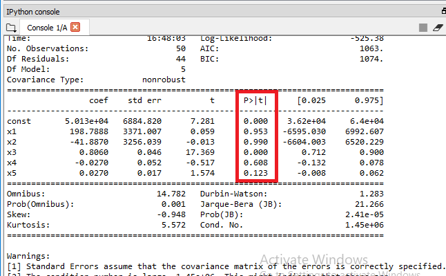
From the output given above, it can be clearly seen that we got P-value for each independent variable. We will now compare the P-value with the significant level (SL=0.05), to decide if we need to remove it from out model or not.
Here x1and x2 is the Dummy Variable, x3 is R&D spend, x4 is Admin spend, and x5 is Marketing spend. We will now look for the highest value of P from the output given above, and we can it is 0.990 or 99% which is way more than the SL value 5%. So, we will need to remove the predictor x2, which is the 2nd Dummy Variable of state.
To remove it, we will perform some of the following steps:
X_opt=X[:, [0,1,3,4,5]]
 regressor_OLS=sm.OLS(endog = Y, exog=X_opt).fit()
 regressor_OLS.summary()
Output:
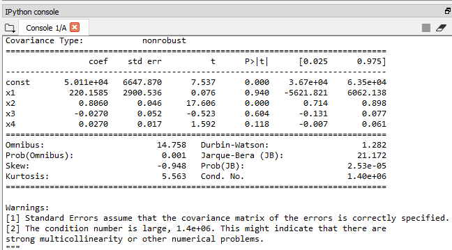
Now the highest value is 94% which is again above than 5% of SL. We will remove x1 which the 1st Dummy Variable of state at index=1 and again perform the same steps to look for next highest P-value until we get the best optimal team to predict the profit.
 X_opt=X[:, [0,3,4,5]]
 regressor_OLS=sm.OLS(endog = Y, exog=X_opt).fit()
 regressor_OLS.summary()
Output:
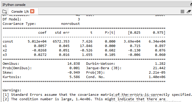
Now the highest P-value is 60%, so we will remove x2which is the Admin spend at index=4 and again check for the highest P-value.
X_opt=X[:, [0,3,5]]
 regressor_OLS=sm.OLS(endog = Y, exog=X_opt).fit()
 regressor_OLS.summary()
Our model is finally getting ready, may be index 3 & 5 which is the Marketing and the R&D spend composed of independent variables makes the best team to predict the profit.
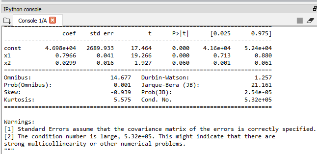
From the output image given above, we need to look at the table and decide the highest P-value. The highest P-value is here 0.060 and 0.000, which is x1. The P-value cannot b0. It’s just so small that it’s way below SL of 5%.
Therefore the R&D spend is a very powerful predictor of profit & definitely has a high statistical impact on the dependent variable profit.
But as far as the 2nd independent variable is concerned, which is the Marketing spend at index 5, the P-value is 0.060, which is slightly above the 5% that we set. So, we need to remove it.
X_opt=X[:, [0,3]]
 regressor_OLS=sm.OLS(endog = Y, exog=X_opt).fit()
 regressor_OLS.summary()
Final Table Output:
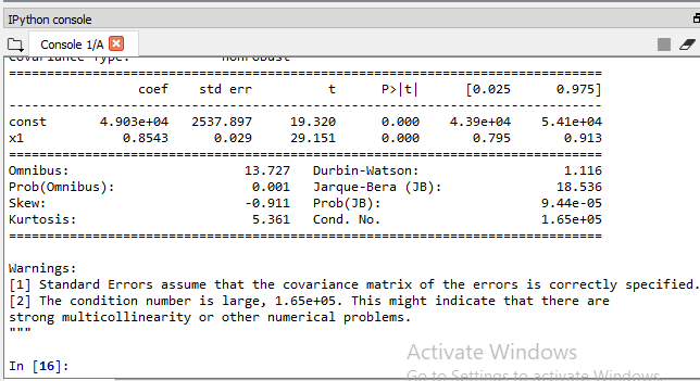
Therefore, it can be seen that the R&D spend variable to make a very powerful predictor of profit. So, finally, the optimal team of the independent variable that can predict profit with the highest statistical significance the strongest impact is composed of only one independent variable i.e., R&D spend.