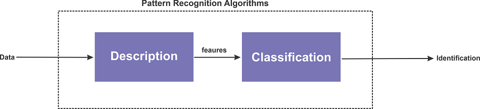
Pattern Recognition and Machine Learning a MATLAB Companion

The cognitive process that occurs in the brain when it compares the information that we see with the information stored in our memories is called pattern recognition. It is what Artificial Intelligence and machine learning aim to imitate in the human brain.

We can also say, “The technique that compares incoming data with data kept in a database is called pattern recognition.” It employs machine learning algorithms to identify patterns, so we can say that it is a form of machine learning.

Below four properties are what pattern recognition and machine learning look for when arranging the attributes of data to provide information about a particular data collection or system:

• It gains insights from data.
• Even when patterns are only partially visible, it instantly detects them.
• It can spot recurring patterns.
• Recognition is based on various forms and angles.

Machine learning and pattern recognition are two sides of the same coin.

Patterns can be found in any type of data. For instance, it can be found in the text, words, images, sounds, miscellaneous data, etc.

Steps for Pattern Recognition

• Data Gathering
• Pre-processing and cleaning the data
• Analysing the information and looking for pertinent characteristics and common factors
• Date grouping and classification
• Analysing data to acquire understanding
• Taking the lessons learned and applying them in real life

Importance Of Pattern Recognition

Pattern recognition increases artificial intelligence by attempting to mimic the neural network capabilities of the human brain. One of the four foundational concepts of computer science is pattern recognition.

In order to find a solution to many real-world computer science-related issues, pattern recognition is required. The key to knowledge is discovering patterns because they represent structure and order, which helps us organize our work and make it more accessible. One of the most important aspects of problem-solving and mathematical reasoning is recognizing and comprehending patterns.

In addition, pattern recognition is important for the following reasons:

• It locates and anticipates even the smallest pieces of concealed or untraceable data.
• It aids in classifying unknown data
• It employs learning techniques to produce useful predictions.
• At different distances, it can recognize and identify an item.
• It can assist in creating useful, actionable recommendations and in forming predictions based on unobserved data.

Machine Learning and Pattern Recognition Techniques

Three separate machine learning and pattern recognition models or methodologies are as follows:

• Statistical Pattern Recognition: This type of pattern recognition uses examples to learn from previous statistical data. The model gathers and analyses data from observations. The model then develops generalization skills by using the rules on fresh observations.

• Syntactic Pattern Recognition: It relies on simpler sub-patterns known as primitives, so this concept is sometimes referred to as structural pattern recognition. Such objects include words, for instance. The linkages between the primitives are referred to as the pattern. To give one example, phrases and texts are created when words (primitives) are connected.

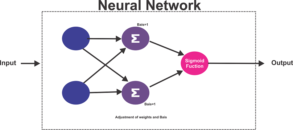
• Neural Pattern Recognition: Artificial neural networks are a component of this paradigm. Complex nonlinear input-output relations are learned by the networks, which then adapt to the data. This approach entails massive parallel computing systems made up of a large number of basic processors and connections between them. They may apply sequential training processes, learn complicated nonlinear input-output relations, and then modify their behavior in response to the data.

Broadly there are two stages of Pattern Recognition and Machine Learning:

• Explorative Stage(Searching for the patterns)
• Descriptive Stage(Categorizing the patterns that were found)

Applications of Machine Learning and Pattern Recognition

The discipline of pattern recognition and machine learning is adaptable and has permeated a wide range of social situations and business sectors. Here are some examples of current applications for pattern recognition and machine learning:

• Stock Market Analysis: The stock market is renowned for its irrationality and volatility. However, it's still possible to spot and capitalize on trends. Applications like Blumberg, Kosho, SofiWealth, and Tinkoff employ artificial intelligence to offer financial advice, supported by pattern detection and machine learning.

• Speech Recognition: Speech recognition algorithms frequently employ words and use them as patterns.

• Geology: The detection and identification of particular types of rocks and minerals may be done by geologists using pattern recognition. To discover, visualize, and analyze temporal patterns in seismic array recordings and create various seismic analysis models, experts may also utilize this technique based on pattern recognition and machine learning.

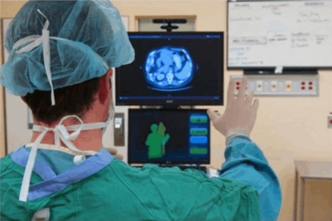
• Medical Diagnosis: Doctors are better able to detect cancer development by utilizing biometric pattern recognition.

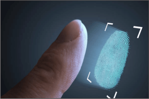
• Fingerprint Scanning: When tracking event attendance or other purposes like it, organizations employ pattern recognition to identify individuals. However, you may probably discover a simpler scanning method right at your fingertips. Fingerprint locks are used on tablets, computers, and smartphones. The unlocking authorization task is taken care of by pattern recognition.

• Engineering: Pattern recognition is widely used by well-known systems like Siri, Alexa, and Google Now.
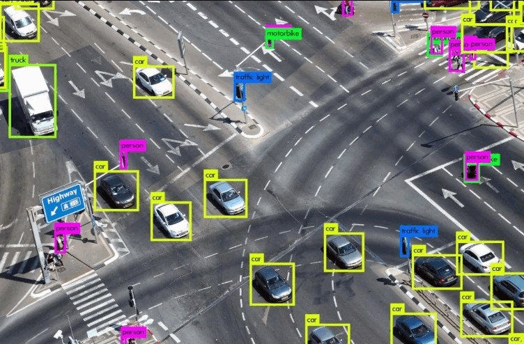
• Computer vision: Single items in photos can be recognized by pattern recognition. To recognize faces, pattern recognition may extract certain patterns from photos or videos. The new patterns are then compared to millions of other photos in the database. Image processing jobs require the human recognition expertise that pattern recognition provides for machines.

• Civil administration: Pattern recognition is used by surveillance and traffic analysis systems to recognize individual cars, trucks, or buses.

MATLAB

For technical computing, MATLAB is a high-performance language. It combines computation, visualization, and programming in a user-friendly setting where issues and answers are presented using well-known mathematical notation.

Which generally include:

• Math and Computation
• Development of Algorithm
• Model building
• Data Analysis
• Exploration and Visualization of data
• Engineering graphs

It is an interactive system with an array as its fundamental data element that doesn't need to be dimensioned. This makes it possible to do many technical computing tasks far faster than it would take to build a program in a scalar noninteractive language like C or Fortran, especially ones using matrix and vector formulations.

Matrix Laboratory is the abbreviation for MATLAB.

Toolboxes are a kind of application-specific solution available in MATLAB. Toolboxes are essential for the majority of MATLAB users since they let you study and use specific technologies. Toolboxes are thorough sets of MATLAB functions (M-files) that enhance the MATLAB environment to address certain issue types. Signal processing, control systems, neural networks, fuzzy logic, wavelets, simulation, and many other fields have toolboxes available.

Pattern Recognition in MATLAB

Cross-validation, data exploration, and classifier construction is made quick and simple by the Pattern Recognition Toolbox for MATLAB, which offers an intuitive and reliable interface to hundreds of pattern classification tools. You have the ability to solve your problem using advanced data analysis methods thanks to PRT. The PRT can help you accomplish more tasks faster if you have data and need to generate predictions using that data.

Here we will look at two pattern recognition with MATLAB:

1. Pizza Puzzle
2. Geometric Transformation Matrix

1. Pizza Puzzle

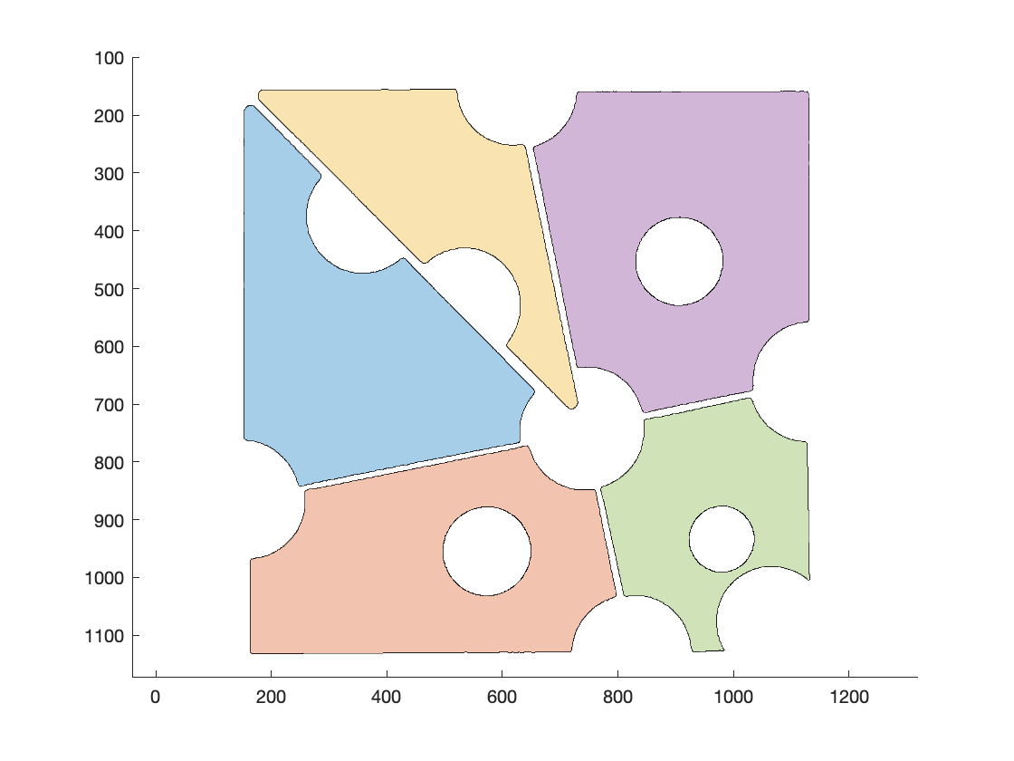
We have to turn the individual "cheese slices" into patch objects for plotting and manipulation.

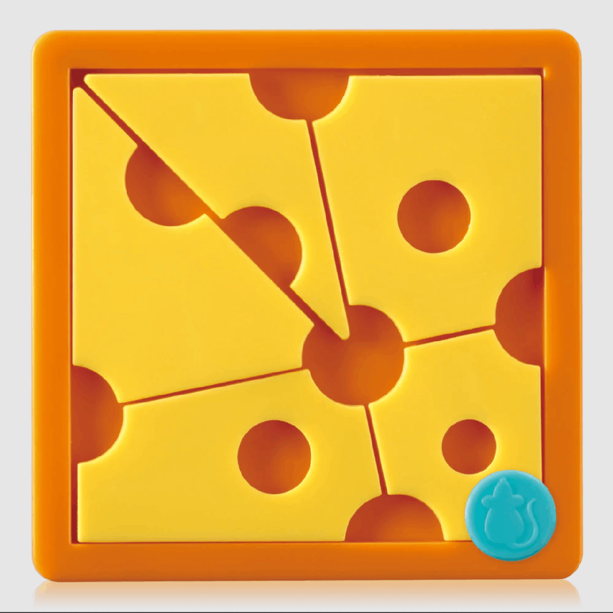
 We have to turn the above image into something like this:

First, we need to use the Color Threshold app to determine some threshold values in CIELAB space.

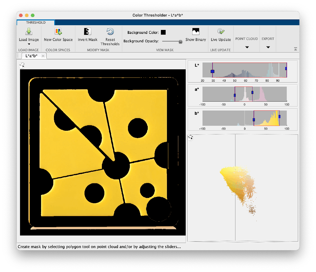
rgb = imread("Cheese_puzzle.png");
lab = rgb2lab(rgb);
% Threshold values chosen with the help of colorThresholder.
[L,a,b] = imsplit(lab);
mask = ((30 <= L) & (L <= 98)) & ...
    ((-20 <= a) & (a <= 16)) & ...
    ((26 <= b) & (b <= 83));
imshow(mask)

Output:

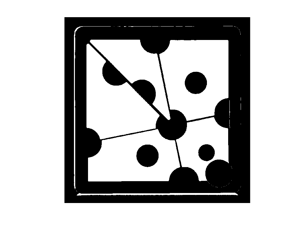
The excess undesired foreground pixels must be removed. Employing a technique known as opening by reconstruction by those who study mathematical morphology.

The first stage is to erode the image so that all the undesirable pixels are removed while at least some of the items we wish to keep are preserved. Thin horizontal lines will be eliminated by erosion by a vertical line, and thin vertical lines will be eliminated by erosion by a horizontal line.

mask2 = imerode(mask,ones(21,1));
imshow(mask2)

Output:

mask3 = imerode(mask2,ones(1,21));
imshow(mask3)

Output:

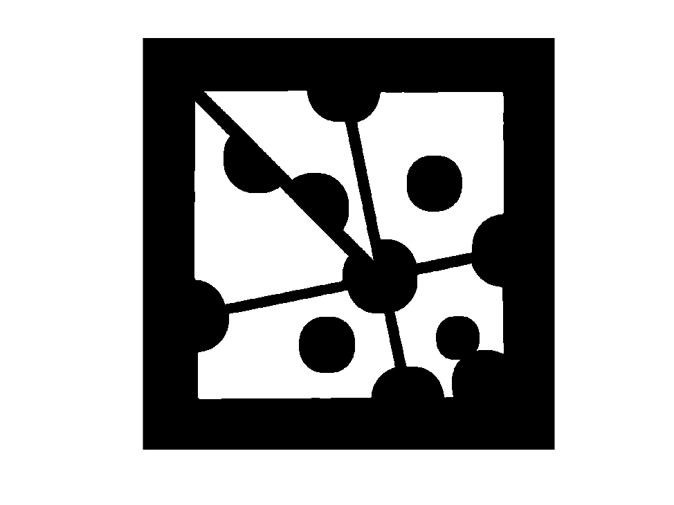
The unnecessary foreground pixels have been removed from the above image, but the jigsaw pieces have shrunk instead. To retrieve all of the jigsaw pieces, we will employ morphological reconstruction.

mask4 = imreconstruct(mask3,mask);
imshow(mask4)

Output:

An object that can represent forms made up of polygons is called a polyshape. A list of polygons that confine distinct regions and holes may be used to form a poly shape, and the Image Processing Toolbox function bwboundaries can generate exactly such a list of polygons.

b = bwboundaries(mask4)

Output:

b = 9×1 cell

	1
1	1820×2 double
2	1687×2 double
3	1669×2 double
4	1771×2 double
5	1328×2 double
6	613×2 double
7	609×2 double
8	457×2 double
9	[472,980;472,980]

The polyshape function can automatically distinguish between polygons that bound areas and those that bound holes from a collection of bounding polygons, however the input arguments for polyshape take a somewhat different format than what bwboundaries generates. Here is some code to change the output of bwboundaries into a format that polyshape can understand.

for k = 1:length(b)
    X{k} = b{k}(:,2);
    Y{k} = b{k}(:,1);
end
ps = polyshape(X,Y)

Output:

ps = 
  polyshape with properties:


      Vertices: [3529×2 double]
    NumRegions: 6
      NumHoles: 3

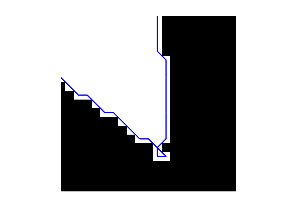
Zooming into of the corners

figure
imshow(mask)
hold on
plot(b{5}(:,2),b{5}(:,1),'b')
hold off
xlim([1120 1140])
ylim([990 1010])

Output:

Divide the polygon into various regions:

ps_regions = regions(ps)

Output:

ps_regions = 
  6×1 polyshape array with properties:


    Vertices
    NumRegions
    NumHoles

Discover each region's area:

region_areas = area(ps_regions)

Output:

region_areas = 6×1
105 ×
    1.7261
    1.5884
    1.0799
    1.9781
    0.9128
    0.0000

Remove the little area:

ps_regions(region_areas < 1) = []

Output:

ps_regions = 
  5×1 polyshape array with properties:


    Vertices
    NumRegions
    NumHoles

We may plan the components of our puzzle. Each polyshape in an array that you supply to the plot will be colored uniquely.

plot(ps_regions)
axis ij
axis equal

Output:

2. Geometric Transformation Matrix

The rigidtform2d, affinetform3d, and other new geometric transformation objects in the Image Processing Toolbox employ the premultiply matrix convention rather than the postmultiply matrix method. Other associated toolbox functions, such imregtform, now favour using these new objects. The premultiply convention and new objects are now used in several methods in the Computer Vision Toolbox and Lidar Toolbox. Additionally, these modifications enhance the Robotics System Toolbox and Navigation Toolbox's design coherence.

Affine Transformation Matrices

The matrices in question describe rigid, rigid, rigid, and similarity transformations as well as affine and projective transformations. In the explanation that follows, we will concentrate on affine transformations, but projective transformations also use the same ideas.

An affine transformation matrix for two dimensions is a 3X3 matrix that use matrix multiplication to transfer the two-dimensional point (u,v) as follows:

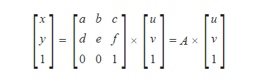
The third row of A is always [001] when the affine transformation is represented as above. We'll refer to this as the premultiply convention because the matrix comes before the vector it is multiplying.

This operation can also be written in another way. Everything may be transposed, like in this:

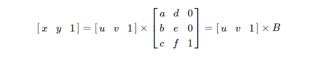
The matrix occurs after the vector in this form, that is why we'll refer to it as the postmultiply convention. Due to matrix transposition, A and B are connected to one another as A= and B= .

Deciding to Change the Convention

Compared to the postmultiply convention, the premultiply convention is now far more common. The premultiply convention is employed by the most widely used information sources, including Wikipedia. Our usage of the postmultiply protocol caused a lot more confusion as a result. This misunderstanding was evident in several MATLAB Answers postings and tech support inquiries. Although it was likely to be challenging and time-consuming, developers on the Image Processing Toolbox and Computer Vision Toolbox teams came to the conclusion that we should try to do something about it.

Latest Geometric Transformation Types

These new types are included in the Image Processing Toolbox R2022b version:

• projtform2d - 2-D projective geometric transformation
• affinetform2d - 2-D affine geometric transformation
• simtform2d - 2-D similarity geometric transformation
• rigidtform2d - 2-D rigid geometric transformation
• transltform2d - 2-D translation geometric transformation
• affinetform3d - 3-D affine geometric transformation
• simtform3d - 3-D similarity geometric transformation
• rigidtform3d - 3-D rigid geometric transformation
• transltform3d - 3-D translation geometric transformation

Utilizing the New Types

The premultiplication form should be used when creating one of the new transformation types from a transformation matrix. The bottom row is [001] for an affine matrix in premultiplication form.

A = [1.5 0 10; 0.1 2 15; 0 0 1]

Output:

A = 3×3
    1.5000         0   10.0000
    0.1000    2.0000   15.0000
         0         0    1.0000

tform = affinetform2d(A)

Output:

tform = 
  affinetform2d with properties:


    Dimensionality: 2
                 A: [3×3 double]

tform.A

Output:

ans = 3×3
    1.5000         0   10.0000
    0.1000    2.0000   15.0000
         0         0    1.0000

The new types are meant to work as seamlessly as feasible with existing code written for the old kinds in order to make the transition easier. Let's look at the outdated function affine2d as an illustration:

T = A'

Output:

T = 3×3
    1.5000    0.1000         0
         0    2.0000         0
   10.0000   15.0000    1.0000

tform_affine2d = affine2d(T)

Output:

tform_affine2d = 
  affine2d with properties:


                 T: [3×3 double]
    Dimensionality: 2

tform_affine2d.T

Output:

ans = 3×3
    1.5000    0.1000         0
         0    2.0000         0
   10.0000   15.0000    1.0000

For the older types, the transformation matrix in postmultiply form is the T property. The premultiplied transformation matrix is the A property for the new kinds.

The transformation matrix in postmultiply form is present in the T property of the new types, which is concealed.

tform

Output:

tform = 
  affinetform2d with properties:


    Dimensionality: 2
                 A: [3×3 double]

tform.A

Output:

ans = 3×3
    1.5000         0  100.0000
    0.1000    2.0000   15.0000
         0         0    1.0000

tform.T

Output:

ans = 3×3
    1.5000    0.1000         0
         0    2.0000         0
  100.0000   15.0000    1.0000

This hidden property enables you to utilize the new type without having to modify any existing code that obtains or sets the T property on the old type. The appropriate A property will be automatically set or obtained when the T property is set or obtained.

tform.T(3,1) = 100;
tform.T

Output:

ans = 3×3
    1.5000    0.1000         0
         0    2.0000         0
  100.0000   15.0000    1.0000

tform.A

Output:

ans = 3×3
    1.5000         0  100.0000
    0.1000    2.0000   15.0000
         0         0    1.0000

Translation and Similarity Transformations

The more specialized transformations translation, stiff, and similarity are included in the new types in addition to the more general affine transformation.

r_tform = rigidtform2d(45,[0.2 0.3])

Output:

r_tform = 
  rigidtform2d with properties:


    Dimensionality: 2
     RotationAngle: 45
       Translation: [0.2000 0.3000]
                 R: [2×2 double]
                 A: [3×3 double]

It is directly calculated from the rotation and translation parameters if you ask for R (the rotation matrix) or A (the affine transformation matrix).

r_tform.R

Output:

ans = 2×2
    0.7071   -0.7071
    0.7071    0.7071

r_tform.A

Output:

ans = 3×3
    0.7071   -0.7071    0.2000
    0.7071    0.7071    0.3000
         0         0    1.0000

These matrices can be changed directly, but only if the outcome would be a legitimate rigid transformation. Because the outcome is still a rigid transformation, the assignment that just modifies the horizontal translation offset is acceptable:

r_tform.A(1,3) = 0.25

Output:

r_tform = 
  rigidtform2d with properties:


    Dimensionality: 2
     RotationAngle: 45
       Translation: [0.2500 0.3000]
                 R: [2×2 double]
                 A: [3×3 double]

Transformation

[x,y] = transformPointsForward(r_tform,2,3)

Output:

x = -0.4571
y = 3.8355

[u,v] = transformPointsInverse(r_tform,x,y)

Output:

u = 2
v = 3

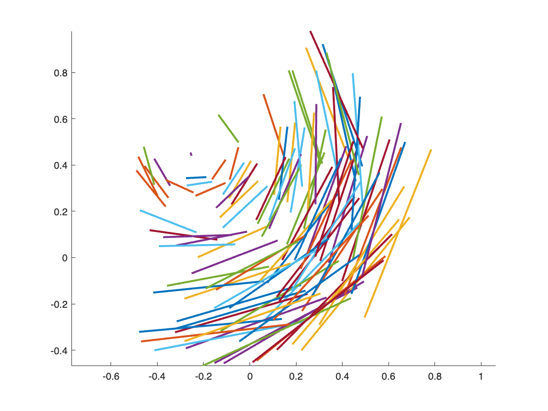
Using the r_tform function from above, the following code creates 100 pairs of random points, transforms them, and then draws line segments connecting the original points to the changed ones.

xy = rand(100,2) - 0.5;
uv = transformPointsForward(r_tform,xy);
clf
hold on
for k = 1:size(xy,1)
    plot([xy(k,1) uv(k,1)],[xy(k,2) uv(k,2)])
end
hold off
axis equal

Output: