Heart Disease Prediction Using Machine Learning

The world uses machine learning in many different fields. This is also true in the healthcare sector. Machine learning may be crucial in determining if locomotor disorders, heart illnesses, and other conditions are present or absent. If anticipated far in advance, such information can provide physicians with insightful knowledge that will enable them to individually tailor each patient's diagnosis and course of treatment.

Here, we'll talk about utilizing machine learning algorithms to identify probable heart diseases in humans.

Dataset

Source: Kaggle

Link: https://www.kaggle.com/code/ayanotemitope/heart-attack-analysis-prediction/data

Problem Defined

Can we determine a patient's risk of heart disease based on clinical parameters?

Data Field

1. age -  years of age of the patient
2. sex -  Gender of the patient ( 0 is for female;  1 is for male)
3. cp - Type of Pain in the chest
4. 0: Typical angina: decreased cardiac blood flow caused by chest discomfort
   • 1: Atypical angina: heart-unrelated chest discomfort
   • 2: Non-anginal pain: esophageal spasms are common (non-heart related)
   • 3: Asymptomatic: chest discomfort not associated with any illness
5. trtbps - blood pressure at rest (in mm Hg on admission to the hospital). Usually, anything between 130 and 140 causes worry.
6. chol - mg/dl of serum cholesterol
   • serum = LDL + HDL + .2 * triglycerides
   • above 200 is cause for concern
7. fbs - (fasting blood sugar > 120 mg/dl) (1 is for true; 0 is for  false)
   • Diabetes is indicated by '>126' mg/dL.
8. restecg - electrocardiograms were taken when at rest
   • 0: Nothing to worry about
   • 1: ST-T Wave abnormality
     1. might range from minor signs to serious issues
     2. signals an irregular heartbeat
   • 2: Whether present or absent, left ventricular hypertrophy
     1. expanded main pumping chamber of the heart
9. thalachh - reached a maximal heart rate
10. exng - Angina brought on by exercise (1  is for yes; 0  is for  no)
11. oldpeak - Exercise-induced ST depression examines the stress on the heart during exercise; a sick heart will stress more.
12. slp - the angle of the ST segment's peak workout
    • 0: Upsloping: exercising causes a higher heart rate (uncommon)
    • 1: Flatsloping: hardly any change (typical healthy heart)
    • 2: Downslopins: indicators of a sick heart
13. caa - main vessels colored with fluoroscopy in number (0–3)
    • The doctor can see the blood flowing via a colored vessel.
    • the more blood movement, the better (no clots)
14. thall - Thallium under stress
    • 1,3: Normal
    • 6: fixed defect: Previously defective, but now ok
    • 7: reversible defect: no normal blood flow when exercising
15. output - Does the patient has a disease or not (1 is for yes, 0 is for no) [ the predicted attribute]

Implementation using Python

Importing Libraries

import pandas as pd
import matplotlib.pyplot as plt
import seaborn as sns
import numpy as np
import hvplot.pandas
from scipy import stats


%matplotlib inline
sns.set_style("whitegrid")
plt.style.use("fivethirtyeight")

Loading the Dataset

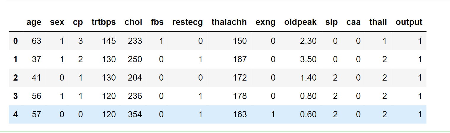
data_ = pd.read_csv("heart.csv")
data_.head()

Output:

EDA (Exploratory Data Analysis)

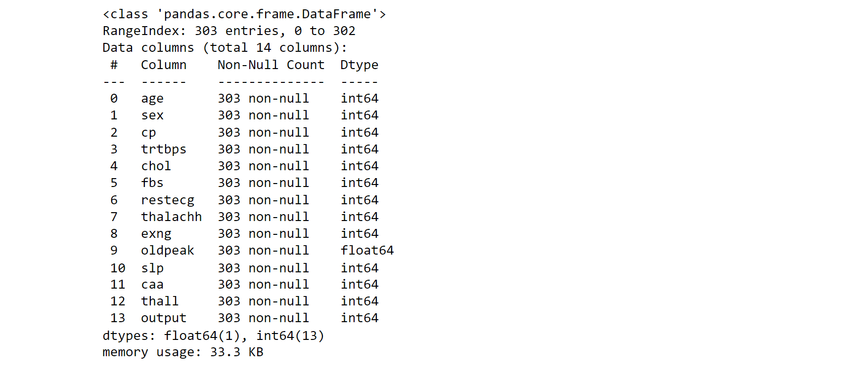
data_.info()

Output:

data_.shape

Output:

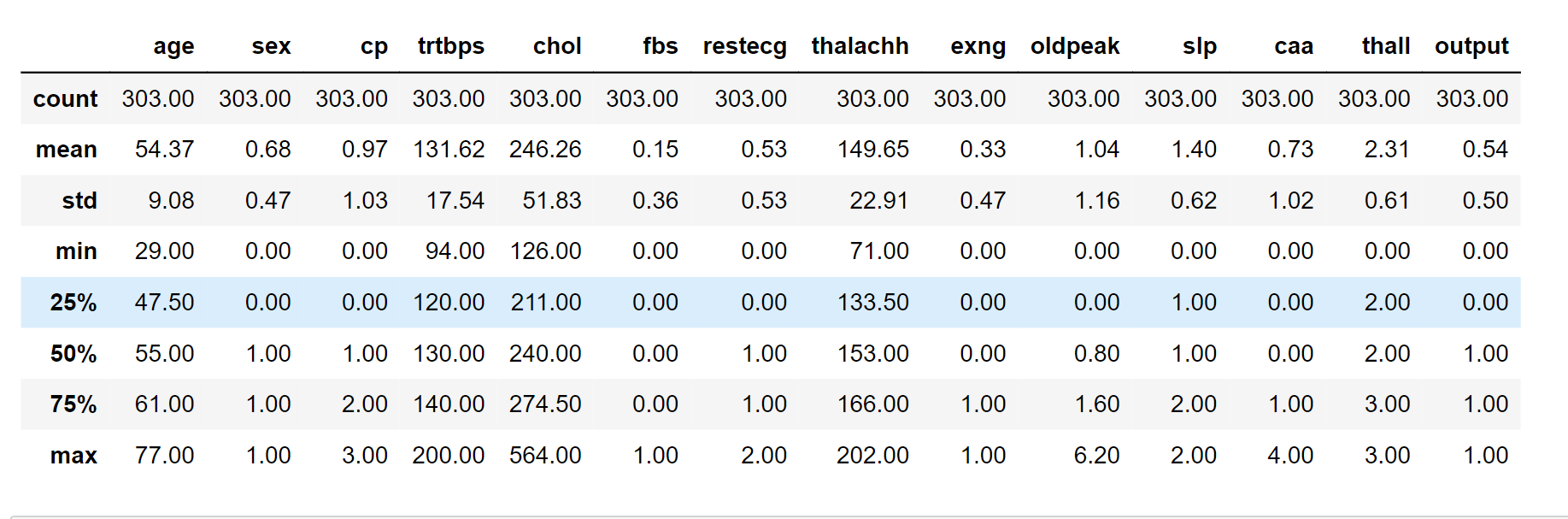
pd.set_option("display.float", "{:.2f}".format)
data_.describe()

Output:

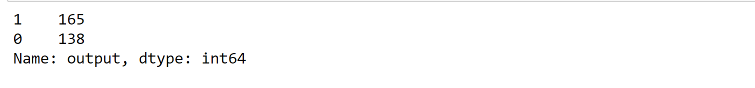
data_.output.value_counts()

Output:

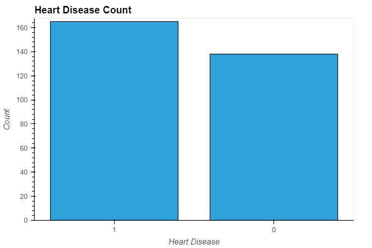
data_.output.value_counts().hvplot.bar(
    title="Heart Disease Count", xlabel='Heart Disease', ylabel='Count',
    width=600, height=400
)

Output:

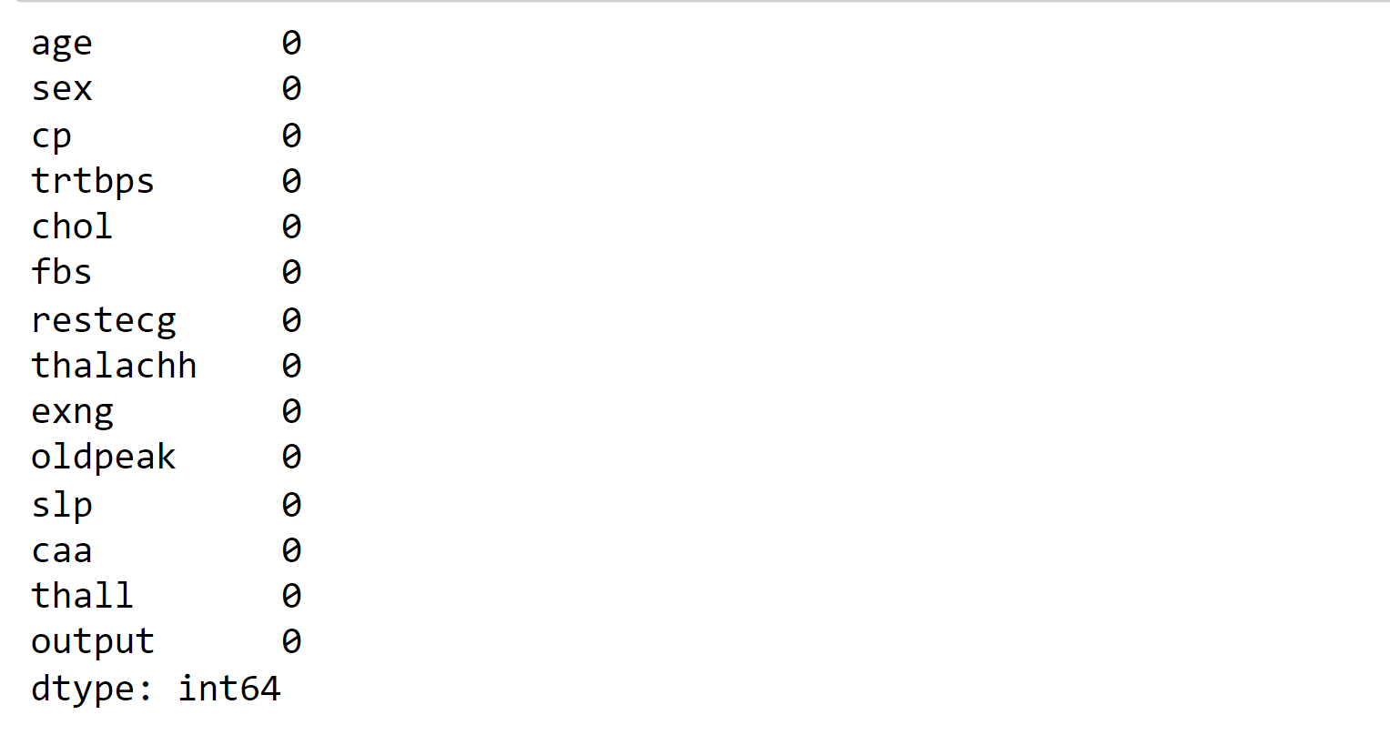
# here, we will check if there is any missing value in our dataset
data_.isna().sum()

Output:

categorical_value = []
continous_value = []
for column in data_.columns:
    if len(data_[column].unique()) <= 10:
        categorical_value.append(column)
    else:
        continous_value.append(column)




categorical_value

Output:

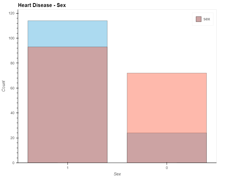
patient_have_disease = data_.loc[data['output']==1, 'sex'].value_counts().hvplot.bar(alpha=0.4)
patient_have_no_disease = data_.loc[data['output']==0, 'sex'].value_counts().hvplot.bar(alpha=0.4)


(patient_have_no_disease * patient_have_disease).opts(
    title="Heart Disease - Sex", xlabel='Sex', ylabel='Count',
    width=700, height=550, legend_cols=2, legend_position='top_right'
)

Output:

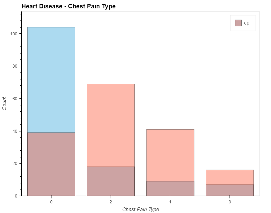
patient_have_disease = data_.loc[data['output']==1, 'cp'].value_counts().hvplot.bar(alpha=0.4)
patient_have_no_disease = data_.loc[data['output']==0, 'cp'].value_counts().hvplot.bar(alpha=0.4)


(patient_have_no_disease * patient_have_disease).opts(
    title="Heart Disease -Chest Pain Type", xlabel='Chest Pain Type', ylabel='Count',
    width=700, height=550, legend_cols=2, legend_position='top_right'
)

Output:

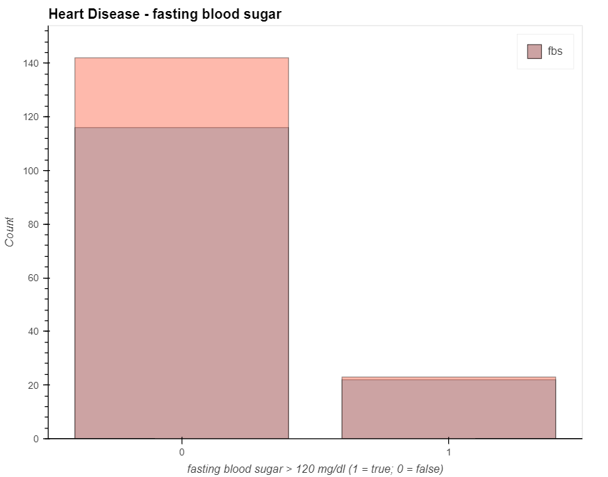
patient_have_disease = data_.loc[data['output']==1, 'fbs'].value_counts().hvplot.bar(alpha=0.4)
patient_have_no_disease = data_.loc[data['output']==0, 'fbs'].value_counts().hvplot.bar(alpha=0.4)


(patient_have_no_disease * patient_have_disease).opts(
    title="Heart Disease - fasting blood sugar", xlabel='fasting blood sugar > 120 mg/dl (1 = true; 0 = false)',
    ylabel='Count', width=700, height=550, legend_cols=2, legend_position='top_right'
)

Output:

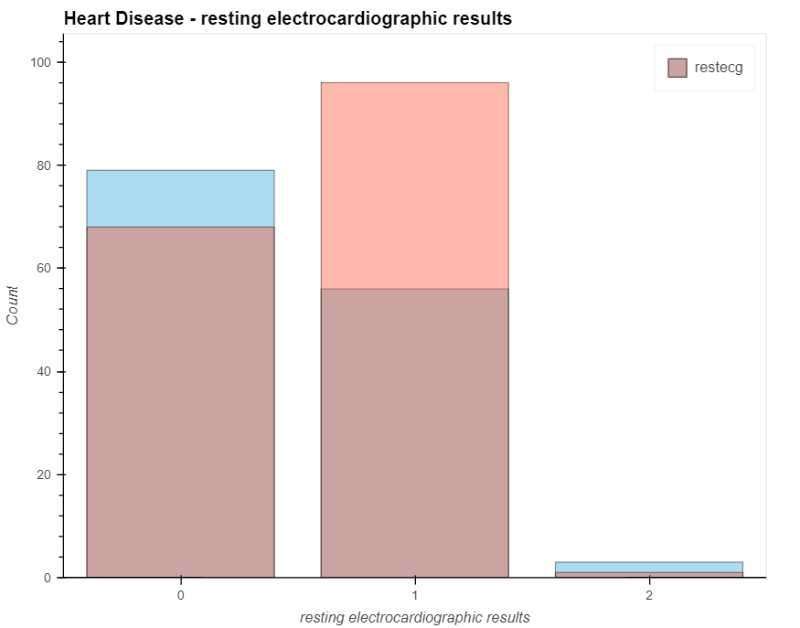
patient_have_disease = data.loc[data['output']==1, 'restecg'].value_counts().hvplot.bar(alpha=0.4)
patient_have_no_disease = data.loc[data['output']==0, 'restecg'].value_counts().hvplot.bar(alpha=0.4)


(patient_have_no_disease * patient_have_disease).opts(
    title="Heart Disease - resting electrocardiographic results", xlabel='resting electrocardiographic results',
    ylabel='Count', width=700, height=550, legend_cols=2, legend_position='top_right'
)

Output:

plt.figure(figsize=(15, 15))


for i, column in enumerate(categorical_val, 1):
    plt.subplot(3, 3, i)
    data_[data_["output"] == 0][column].hist(bins=35, color='blue', label='Have Heart Disease = NO', alpha=0.6)
    data_[data_["output"] == 1][column].hist(bins=35, color='red', label='Have Heart Disease = YES', alpha=0.6)
    plt.legend()
    plt.xlabel(column)

Output:

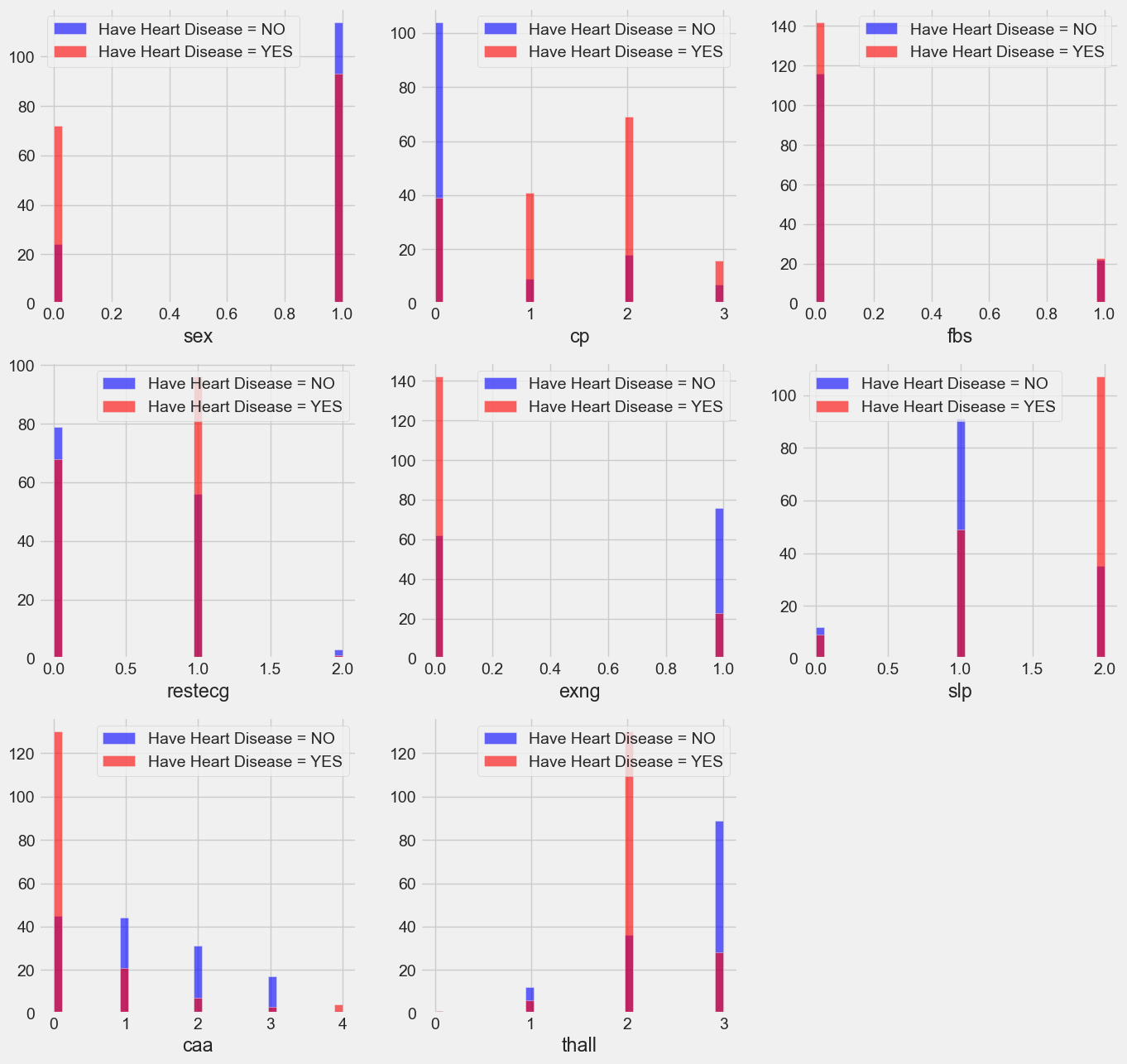
From above, we can conlcude following observations for Heart disease:

• People with a chest pain score of 1, 2, or 3 are more likely to develop heart disease than those with a score of 0.
• People with value 1 (signals non-normal heart rhythm, can vary from moderate symptoms to serious difficulties) on their resting electrocardiogram are more likely to develop heart disease.
• Exercise-induced angina (exng): Those who score 0 (no ==> exercise-induced angina) are more likely to suffer heart disease than those who score 1 (yes ==> exercise-induced angina).
• People with slope values of 2 (signs of an unhealthy heart) are more likely to develop heart disease than those with slope values of 0 (better heart rate with exercise) or 1 (minimal change, typical healthy heart), according to studies. The slope of the ST section of the peak workout.
• People with a ca value of 0 are more prone to develop heart problems because the greater blood flow, measured by the number of main arteries (0–3) colored with fluoroscopy, the better.
• Thallium stress result: Individuals with that value of 2 (fixed defect: formerly defective but now ok) are more prone to develop heart disease.

plt.figure(figsize=(15, 15))


for i, column in enumerate(continous_val, 1):
    plt.subplot(3, 2, i)
    data_[data_["output"] == 0][column].hist(bins=35, color='blue', label='Have Heart Disease = NO', alpha=0.6)
    data_[data_["output"] == 1][column].hist(bins=35, color='red', label='Have Heart Disease = YES', alpha=0.6)
    plt.legend()
    plt.xlabel(column)

Output:

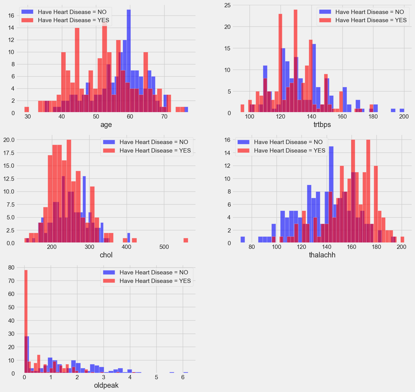
• Resting blood pressure: trstbps (on admission to the hospital, in mm Hg). Usually, anything between 130 and 140 causes worry.
• A serum cholesterol level of 200 or above warrants caution.
• A person who has reached a maximal heart rate of greater than 140 is more likely to suffer heart disease.
• Outdated ST Depression brought on by exercise compared to rest examines the heart's stress levels during activity; a sick heart will stress more.

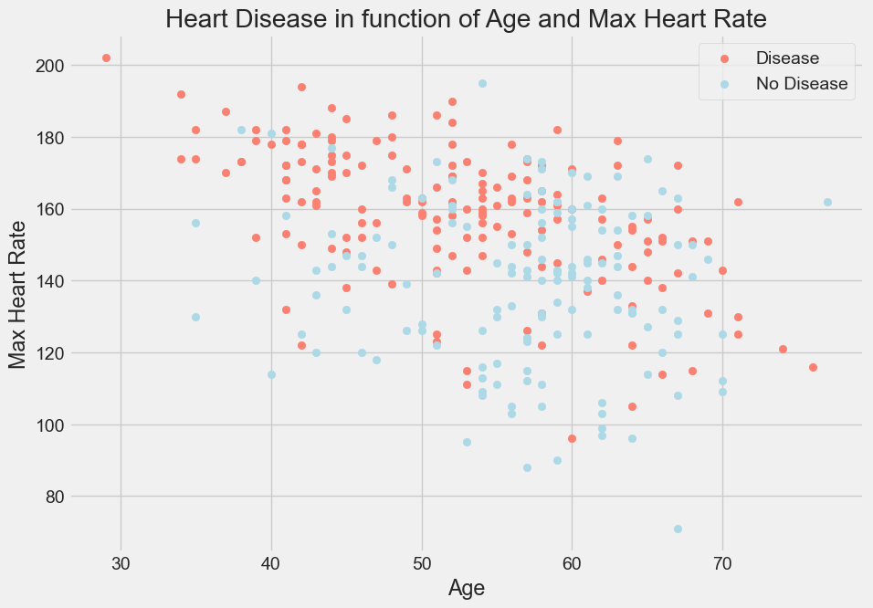
Max Heart Rate versus Age for Heart Disease

# Creating Different figure
plt.figure(figsize=(10, 7))


# Scattering with positive references
plt.scatter(data_.age[data_.output==1],
            data_.thalachh[data_.output==1],
            c="salmon")


# Scattering with negative references
plt.scatter(data_.age[data_.output==0],
            data_.thalachh[data_.output==0],
            c="lightblue")


# Info for ease
plt.title("Heart Disease in function of Max Heart Rate and Age")
plt.xlabel("Age - Age of the Patient")
plt.ylabel("Max Heart Rate - Maximum Heart Rate of the Patient")
plt.legend(["Disease", "No-Disease"]);

Output:

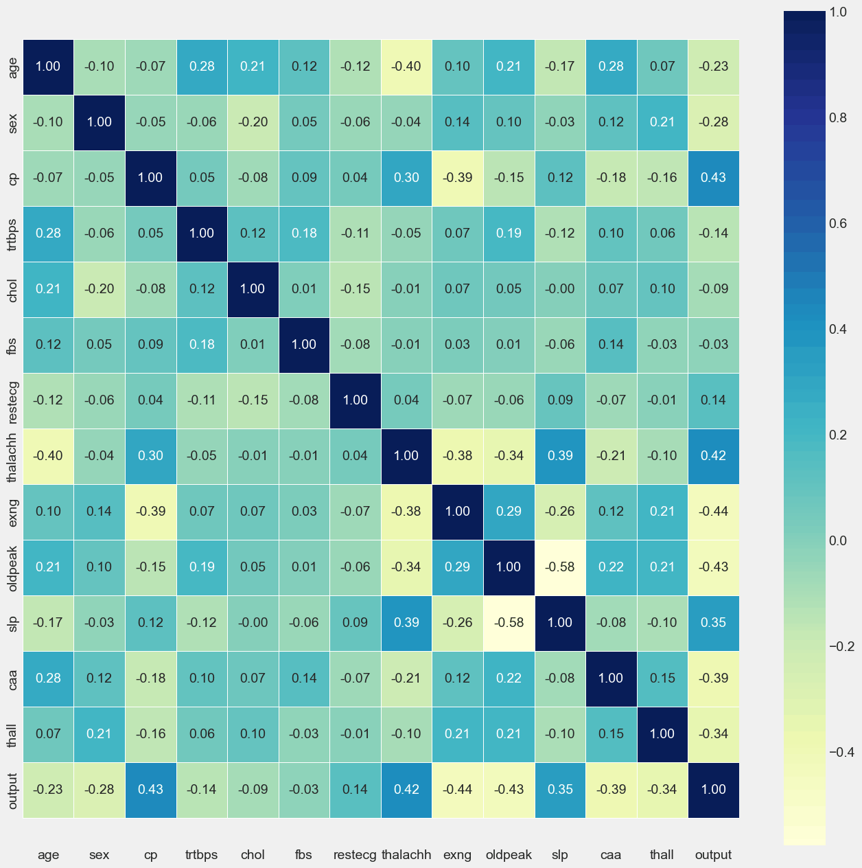
Correlation Matrix

corr_matrix = data_.corr()
fig, ax = plt.subplots(figsize=(15, 15))
ax = sns.heatmap(corr_matrix,
                 annot=True,
                 linewidths=0.5,
                 fmt=".2f",
                 cmap="YlGnBu");
bottom, top = ax.get_ylim()
ax.set_ylim(bottom + 0.5, top - 0.5)

Output:

data_.drop('output', axis=1).corrwith(data_.output).hvplot.barh(
    width=800, height=600,
    title="Correlation between Numeric Features and Heart Disease",
    ylabel='Correlation', xlabel='Numerical Features',
)

Output:

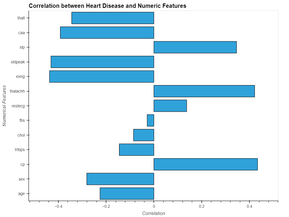
• The output variable has the lowest correlations with fbs and chol.
• The output variable and all other variables are significantly correlated.

Processing of Data

Before training the machine learning models, we must scale all the values after examining the dataset and change certain category variables into dummy variables.

categorical_value.remove('output')
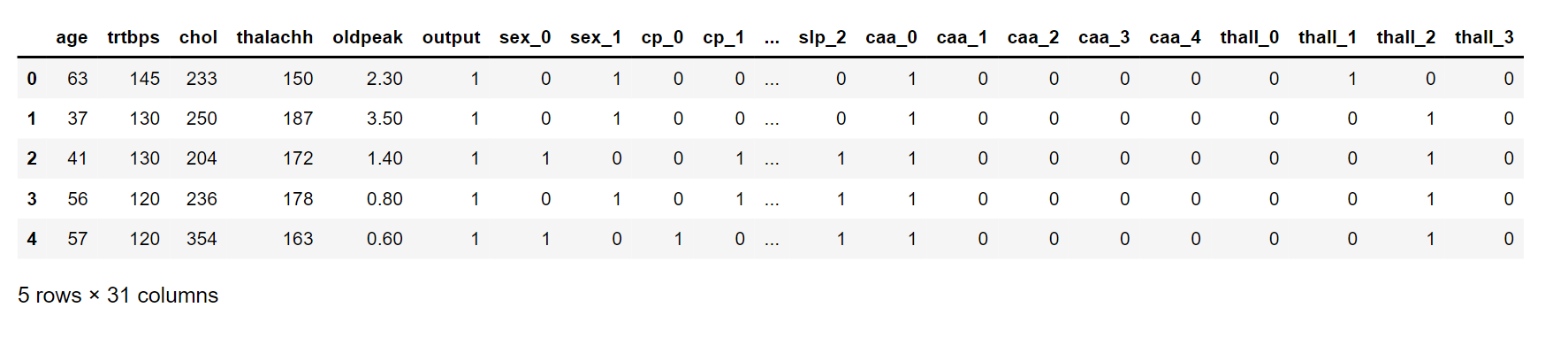
dataset = pd.get_dummies(data_, columns = categorical_value)


dataset.head()

Output:

print(data.columns)
print(dataset.columns)

Output:

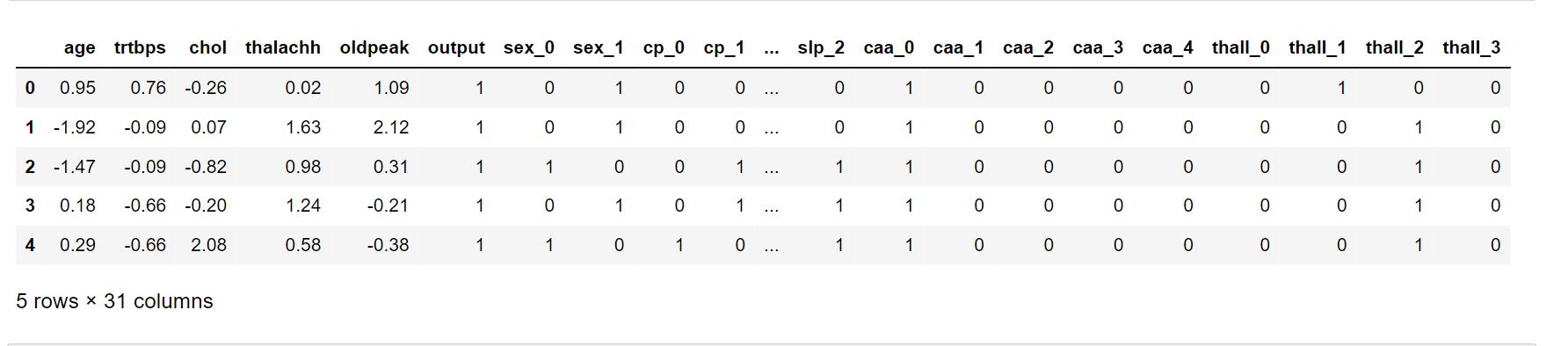
from sklearn.preprocessing import StandardScaler


ssc = StandardScaler()
scale_col = ['age', 'trtbps', 'chol', 'thalachh', 'oldpeak']
dataset[scale_col] = ssc.fit_transform(dataset[col_to_scale])


dataset.head()

Output:

Building Models

from sklearn.metrics import accuracy_score, confusion_matrix, classification_report


def printing_score(classifier, X_train, y_train, X_test, y_test, train=True):
    if train==True:
        prediction = classifier.predict(X_train)
        report = pd.DataFrame(classification_report(y_train, prediction, output_dict=True))
        print(" Result - Train :\n-------------------------------------------")
        print(f"Score for Accuracy: {accuracy_score(y_train, prediction) * 100:.2f}%")
        print("-----------------------------------------------")
        print(f"Report of Classification:\n{report}")
        print("------------------------------------------------")
        print(f"Confusion Matrix: \n {confusion_matrix(y_train, prediction)}\n")
       
    elif train==False:
        prediction = classifier.predict(X_test)
        report = pd.DataFrame(classification_report(y_test, prediction, output_dict=True))
        print("Test Result:\n-----------------------------------------------------")        
        print(f"Score for Accuracy: {accuracy_score(y_test, prediction) * 100:.2f}%")
        print("-----------------------------------------------")
        print(f"Report of Classification:\n{report}")
        print("------------------------------------------------")
        print(f"Confusion Matrix: \n {confusion_matrix(y_test, prediction)}\n")

Here, we will split our data into two: Train Dataset and Testing Dataset

from sklearn.model_selection import train_test_split


X = dataset.drop('output', axis=1)
y = dataset.output


X_train, X_test, y_train, y_test = train_test_split(X, y, test_size=0.3, random_state=42)

We will try different Machine Learning models.

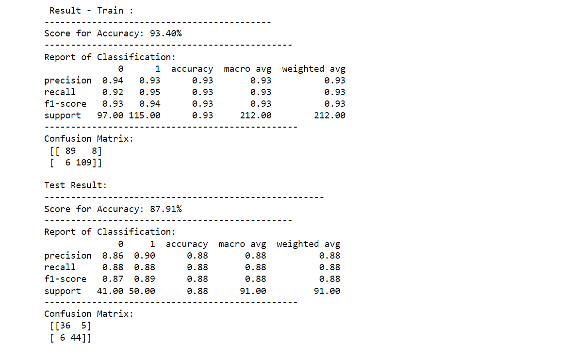
1. Logistic Regression

from sklearn.linear_model import LogisticRegression


logistic_regression_classification = LogisticRegression(solver='liblinear')
logistic_regression_classification.fit(X_train, y_train)


printing_score(logistic_regression_classification , X_train, y_train, X_test, y_test, train=True)
printing_score(logistic_regression_classification , X_train, y_train, X_test, y_test, train=False)

Output:

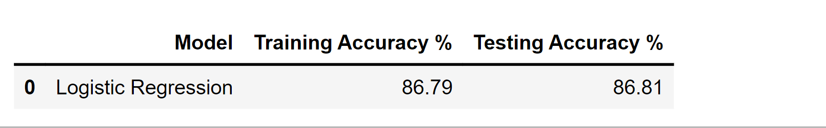
score_test = accuracy_score(y_test, logistic_regression_classification.predict(X_test)) * 100
score_train = accuracy_score(y_train, logistic_regression_classification.predict(X_train)) * 100


df_result = pd.DataFrame(data=[["Logistic Regression", score_train, score_test]],
                          columns=['Model', 'Training Accuracy %', 'Testing Accuracy %'])
df_result

Output:

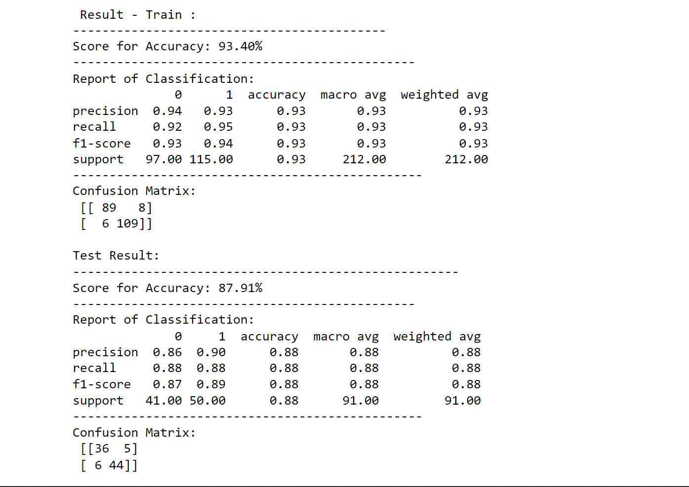
2. Support Vector Machine (SVM)

from sklearn.svm import SVC




svm_classification = SVC(kernel='rbf', gamma=0.1, C=1.0)
svm_classification.fit(X_train, y_train)


printing_score(svm_classification, X_train, y_train, X_test, y_test, train=True)
printing_score(svm_classification, X_train, y_train, X_test, y_test, train=False)

Output:

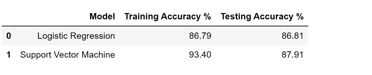
test_score = accuracy_score(y_test, svm_clf.predict(X_test)) * 100
train_score = accuracy_score(y_train, svm_clf.predict(X_train)) * 100


results_df_2 = pd.DataFrame(data=[["Support Vector Machine", train_score, test_score]],
                          columns=['Model', 'Training Accuracy %', 'Testing Accuracy %'])
results_df = results_df.append(results_df_2, ignore_index=True)
results_df

Output:

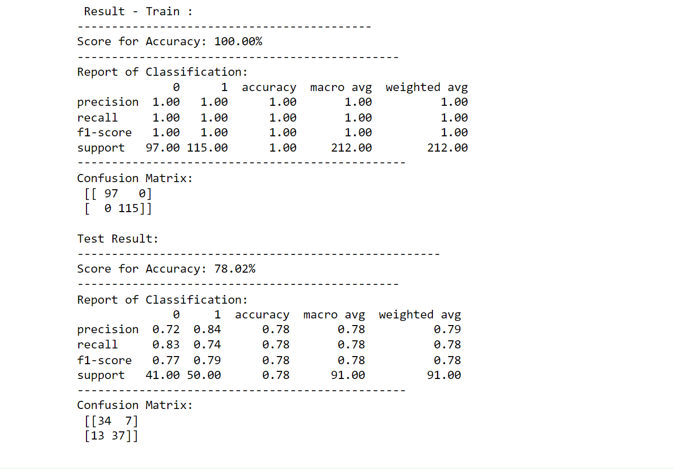
3. Decision Tree Classifier

from sklearn.tree import DecisionTreeClassifier




tree_classification = DecisionTreeClassifier(random_state=42)
tree_classification.fit(X_train, y_train)


printing_score(tree_classification, X_train, y_train, X_test, y_test, train=True)
printing_score(tree_classification, X_train, y_train, X_test, y_test, train=False)

Output:

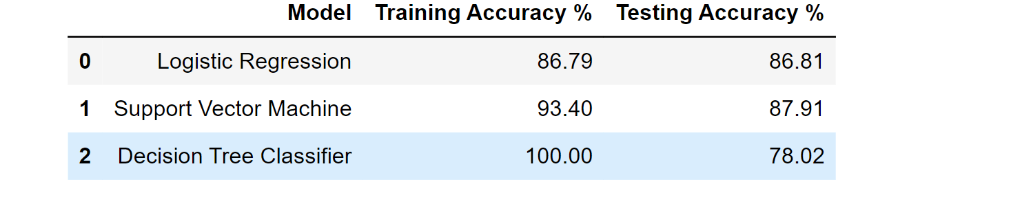
score_test = accuracy_score(y_test, tree_classification.predict(X_test)) * 100
score_train = accuracy_score(y_train, tree_classification.predict(X_train)) * 100


result = pd.DataFrame(data=[["Decision Tree Classifier", score_train, score_test]],
                          columns=['Model', 'Training Accuracy %', 'Testing Accuracy %'])
df_result = df_result.append(result, ignore_index=True)
df_result

Output:

4. Random Forest Classifier

from sklearn.ensemble import RandomForestClassifier
from sklearn.model_selection import RandomizedSearchCV


random_f_classification = RandomForestClassifier(n_estimators=1000, random_state=42)
random_f_classification.fit(X_train, y_train)


printing_score(random_f_classification, X_train, y_train, X_test, y_test, train=True)
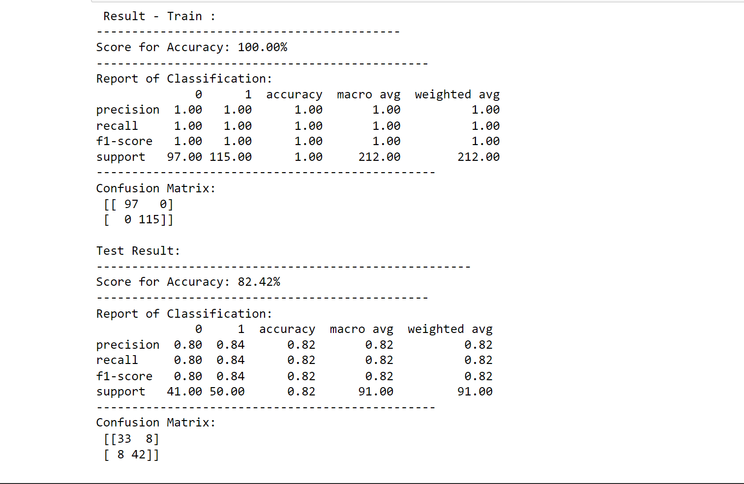
printing_score(random_f_classification, X_train, y_train, X_test, y_test, train=False)

Output:

score_test = accuracy_score(y_test, random_f_classification.predict(X_test)) * 100
score_train = accuracy_score(y_train, random_f_classification.predict(X_train)) * 100


result = pd.DataFrame(data=[["Random Forest Classifier", score_train, score_test]],
                          columns=['Model', 'Training Accuracy %', 'Testing Accuracy %'])
df_result = df_result.append(result, ignore_index=True)
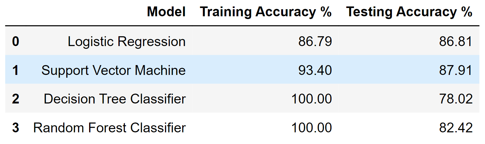
df_result

Output:

5. XGBoost Classifier

from xgboost import XGBClassifier


xgb_classifier = XGBClassifier(use_label_encoder=False)
xgb_classifier.fit(X_train, y_train)


printing_score(xgb_classifier, X_train, y_train, X_test, y_test, train=True)
printing_score(xgb_classifier, X_train, y_train, X_test, y_test, train=False)

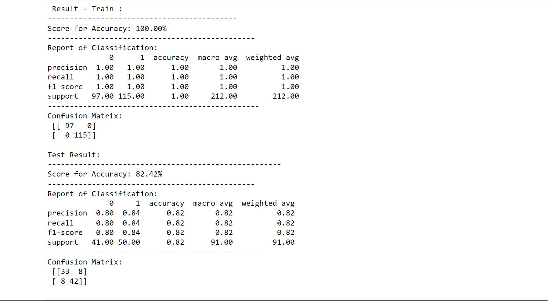
Output:

score_test = accuracy_score(y_test, xgb_classifier.predict(X_test)) * 100
score_train = accuracy_score(y_train, xgb_classifier.predict(X_train)) * 100


result = pd.DataFrame(data=[["XGBoost Classifier", score_train, score_test]],
                          columns=['Model', 'Training Accuracy %', 'Testing Accuracy %'])
df_result = df_result.append(result, ignore_index=True)
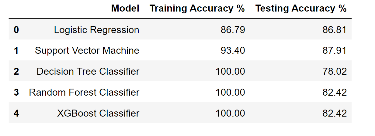
df_result

Output:

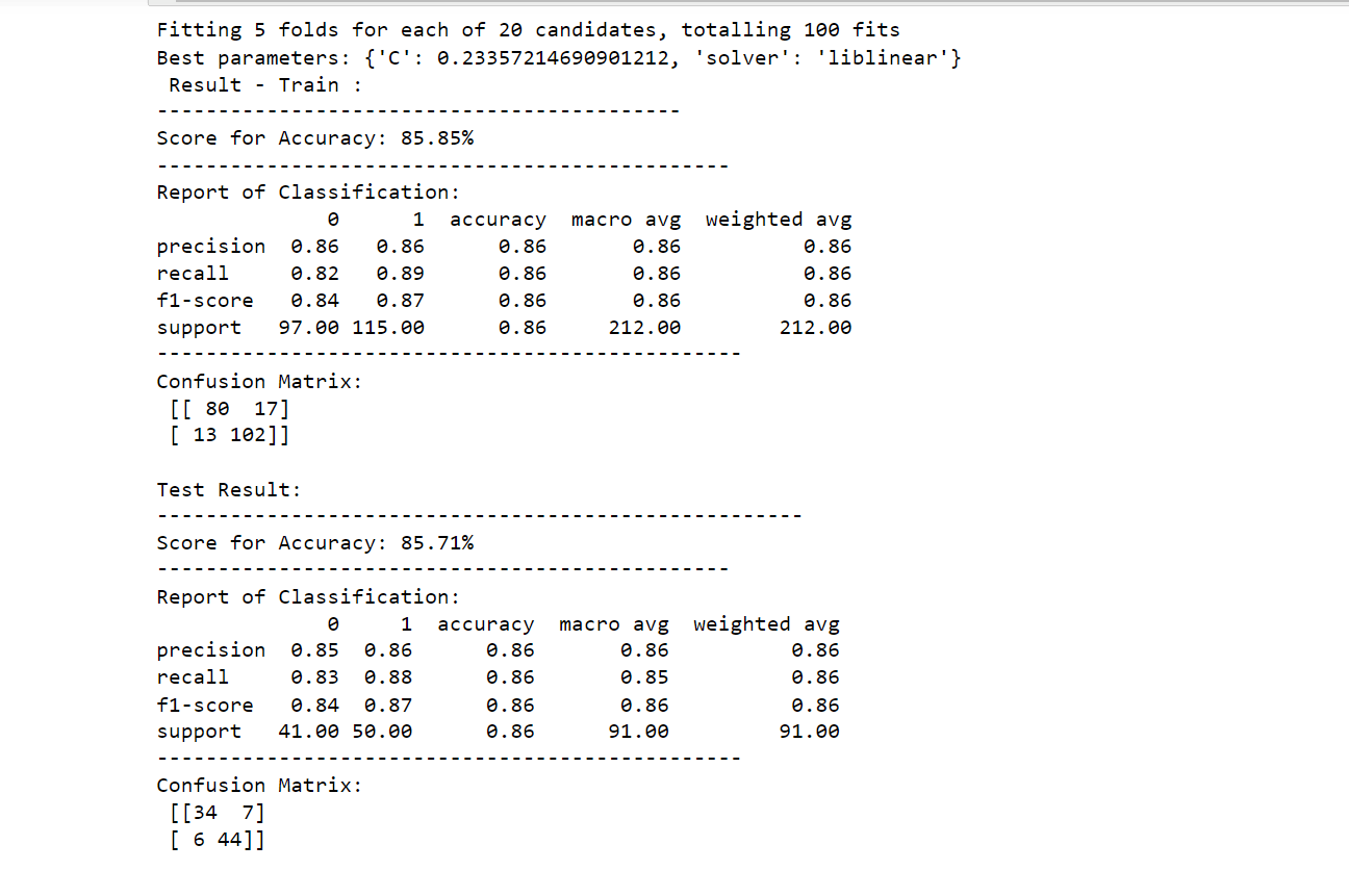
Hyperparameter Tuning of Models

1. Logistic Regression Hyperparameter Tuning

from sklearn.model_selection import GridSearchCV


params = {"C": np.logspace(-4, 4, 20),
          "solver": ["liblinear"]}


logictic_regression_classification = LogisticRegression()


logistic_regression_cv = GridSearchCV(logictic_regression_classification, params, scoring="accuracy", n_jobs=-1, verbose=1, cv=5)
logistic_regression_cv.fit(X_train, y_train)
best_params = logistic_regression_cv.best_params_
print(f"Best parameters: {best_params}")
logictic_regression_classification = LogisticRegression(**best_params)


logictic_regression_classification.fit(X_train, y_train)


printing_score(logictic_regression_classification, X_train, y_train, X_test, y_test, train=True)
printing_score(logictic_regression_classification, X_train, y_train, X_test, y_test, train=False)

Output:

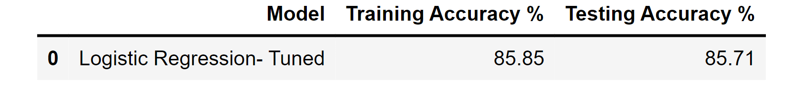
score_test = accuracy_score(y_test, logistic_regression_classifier.predict(X_test)) * 100
score_train = accuracy_score(y_train, logistic_regression_classifier.predict(X_train)) * 100


df_result_tuned = pd.DataFrame(data=[[" Logistic Regression- Tuned", score_train, score_test]],
                          columns=['Model', 'Training Accuracy %', 'Testing Accuracy %'])
df_result_tuned

Output:

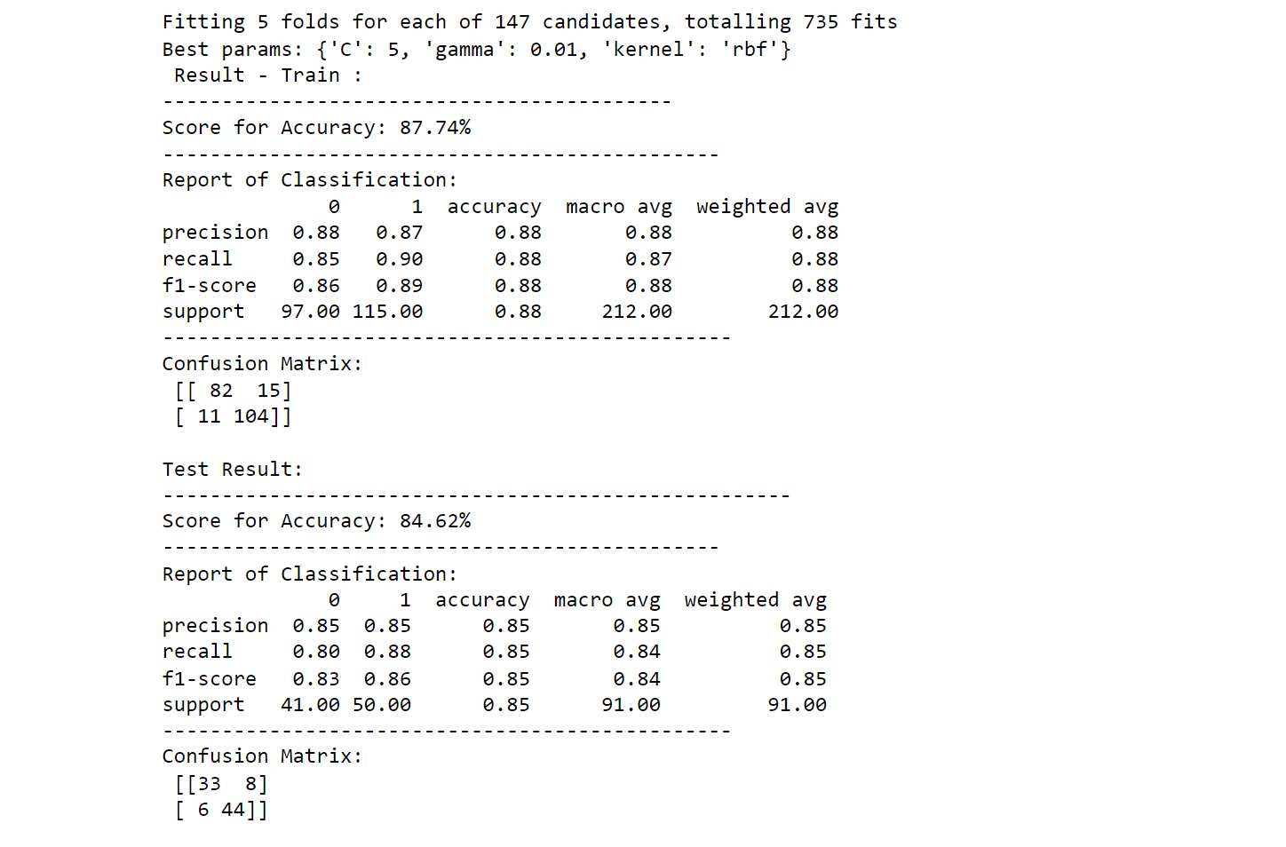
2.  Support Vector Machine(SVM) Hyperparameter Tuning

svm_classifier = SVC(kernel='rbf', gamma=0.1, C=1.0)


params = {"C":(0.1, 0.5, 1, 2, 5, 10, 20),
          "gamma":(0.001, 0.01, 0.1, 0.25, 0.5, 0.75, 1),
          "kernel":('linear', 'poly', 'rbf')}


svm_cv_ = GridSearchCV(svm_classifier, params, n_jobs=-1, cv=5, verbose=1, scoring="accuracy")
svm_cv_.fit(X_train, y_train)
best_params_ = svm_cv_.best_params_
print(f"Best params: {best_params_}")


svm_classifier = SVC(**best_params_)
svm_classifier.fit(X_train, y_train)


printing_score(svm_classifier, X_train, y_train, X_test, y_test, train=True)
printing_score(svm_classifier, X_train, y_train, X_test, y_test, train=False)

Output:

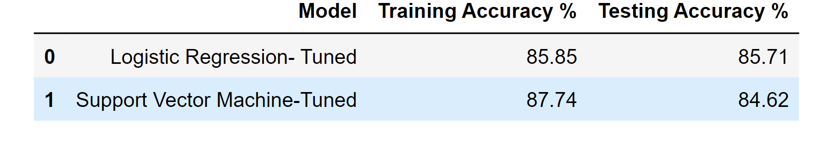
score_test = accuracy_score(y_test, svm_classifier.predict(X_test)) * 100
score_train = accuracy_score(y_train, svm_classifier.predict(X_train)) * 100


result = pd.DataFrame(data=[[" Support Vector Machine-Tuned", score_train, score_test]],
                          columns=['Model', 'Training Accuracy %', 'Testing Accuracy %'])
df_result_tuned = df_result_tuned.append(result, ignore_index=True)
df_result_tuned

Output:

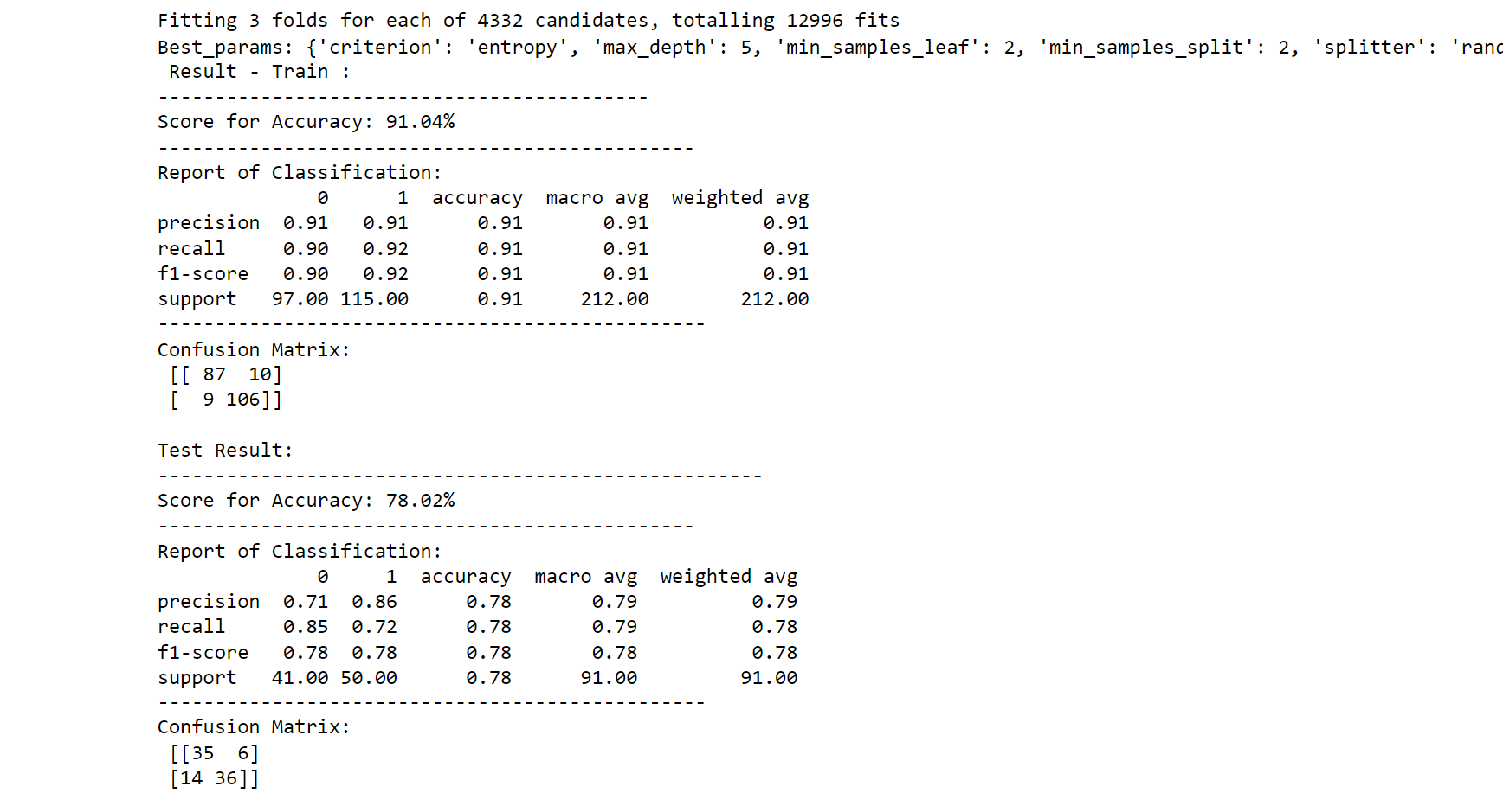
3. Decision Tree Classifier Hyperparameter Tuning

params = {"criterion":("gini", "entropy"),
          "splitter":("best", "random"),
          "max_depth":(list(range(1, 20))),
          "min_samples_split":[2, 3, 4],
          "min_samples_leaf":list(range(1, 20))
          }


dtree_classifier = DecisionTreeClassifier(random_state=42)
dtree_cv = GridSearchCV(dtree_classifier, params, scoring="accuracy", n_jobs=-1, verbose=1, cv=3)
dtree_cv.fit(X_train, y_train)
best_params_ = dtree_cv.best_params_
print(f'Best_params: {best_params_}')


dtree_classifier = DecisionTreeClassifier(**best_params_)
dtree_classifier.fit(X_train, y_train)


printing_score(dtree_classifier, X_train, y_train, X_test, y_test, train=True)
printing_score(dtree_classifier, X_train, y_train, X_test, y_test, train=False)

Output:

score_test = accuracy_score(y_test, dtree_classifier.predict(X_test)) * 100
score_train = accuracy_score(y_train, dtree_classifier.predict(X_train)) * 100


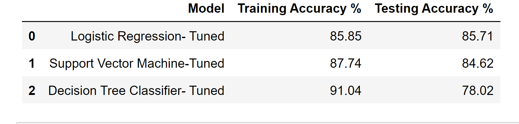
result = pd.DataFrame(data=[[" Decision Tree Classifier- Tuned", score_train, score_test]],
                          columns=['Model', 'Training Accuracy %', 'Testing Accuracy %'])
df_result_tuned = df_result_tuned.append(result, ignore_index=True)
df_result_tuned

Output:

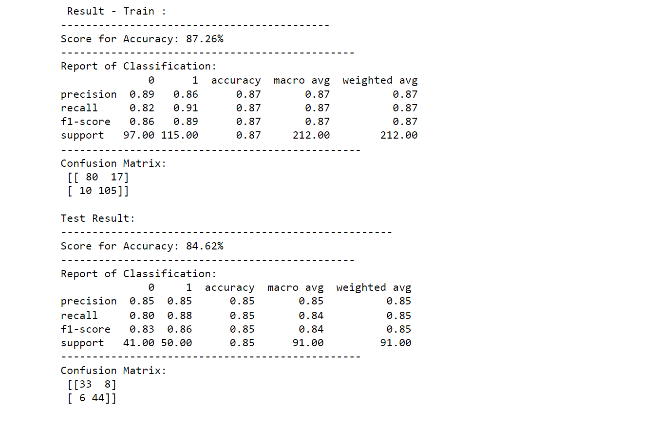
4. Random Forest Classifier Hyperparameter Tuning

n_estimators = [500, 900, 1100, 1500]
max_features = ['auto', 'sqrt']
max_depth = [2, 3, 5, 10, 15, None]
min_samples_split = [2, 5, 10]
min_samples_leaf = [1, 2, 4]


params_grid = {
    'n_estimators': n_estimators,
    'max_features': max_features,
    'max_depth': max_depth,
    'min_samples_split': min_samples_split,
    'min_samples_leaf': min_samples_leaf
              }


random_forest_classifier = RandomForestClassifier(random_state=42)
random_forest_cv = GridSearchCV(random_forest_classifier, params_grid, scoring="accuracy", cv=3, verbose=1, n_jobs=-1)
random_forest_cv.fit(X_train, y_train)
best_params_ = random_forest_cv.best_params_
print(f"Best parameters: {best_params_}")


random_forest_classifier = RandomForestClassifier(**best_params_)
random_forest_classifier.fit(X_train, y_train)




printing_score(random_forest_classifier, X_train, y_train, X_test, y_test, train=True)
printing_score(random_forest_classifier, X_train, y_train, X_test, y_test, train=False)

Output:

score_test = accuracy_score(y_test, random_forest_classifier.predict(X_test)) * 100
score_train = accuracy_score(y_train, random_forest_classifier.predict(X_train)) * 100


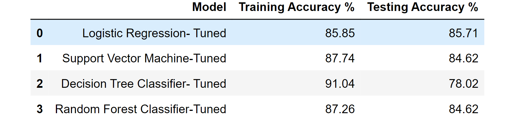
result = pd.DataFrame(data=[["Random Forest Classifier-Tuned", score_train, score_test]], 
                          columns=['Model', 'Training Accuracy %', 'Testing Accuracy %'])
df_result_tuned = df_result_tuned.append(result, ignore_index=True)
df_result_tuned

Output:

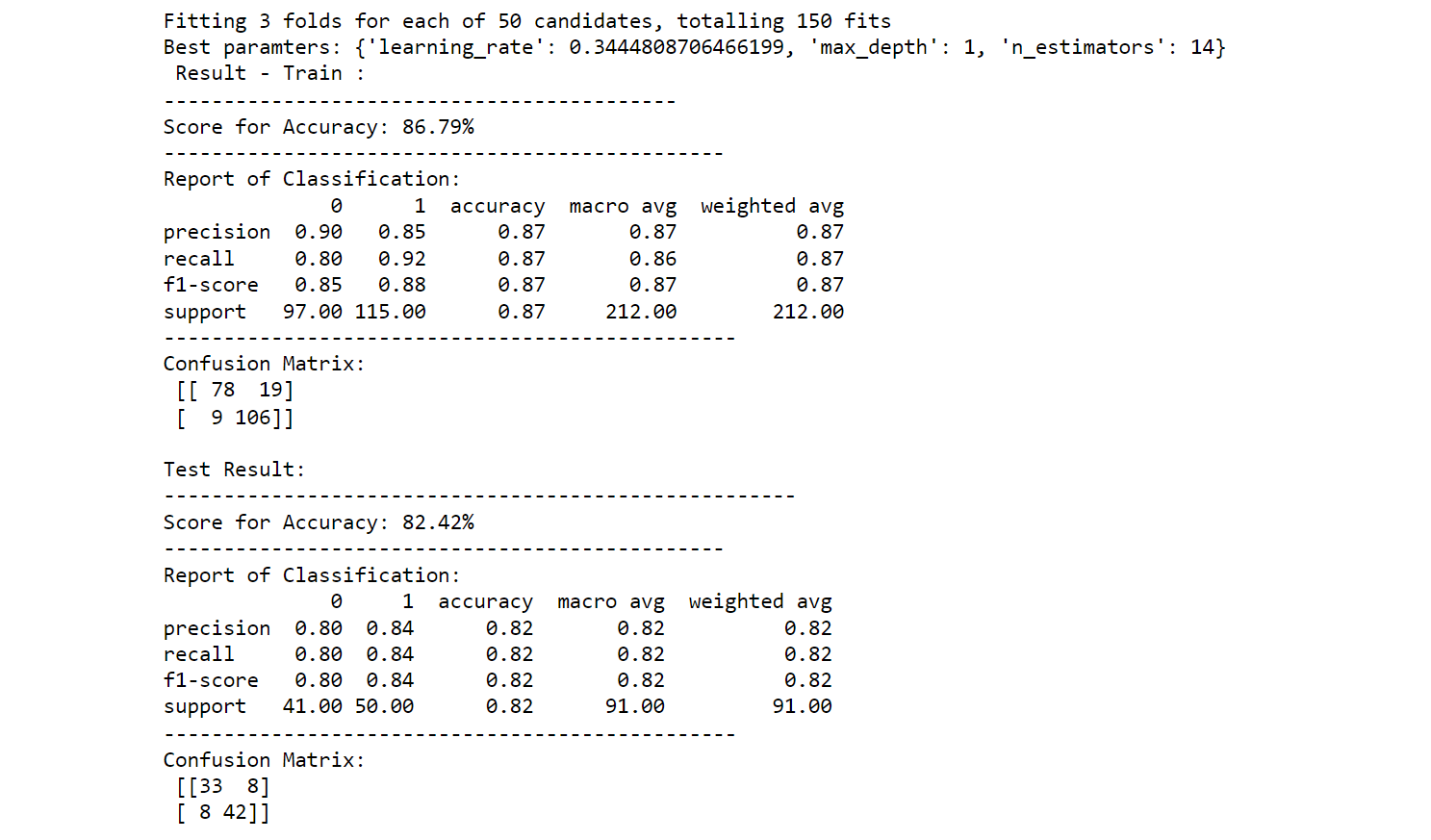
5. XGBoost Classifier Hyperparameter Tuning

param_grid = dict(
    n_estimators=stats.randint(10, 1000),
    max_depth=stats.randint(1, 10),
    learning_rate=stats.uniform(0, 1)
)


xgb_classifier = XGBClassifier(use_label_encoder=False)
xgboost_cv = RandomizedSearchCV(
    xgb_classifier, param_grid, cv=3, n_iter=50,
    scoring='accuracy', n_jobs=-1, verbose=1
)
xgboost_cv.fit(X_train, y_train)
best_params_ = xgboost_cv.best_params_
print(f"Best paramters: {best_params_}")


xgb_classifier = XGBClassifier(**best_params_)
xgb_classifier.fit(X_train, y_train)


printing_score(xgb_classifier, X_train, y_train, X_test, y_test, train=True)
printing_score(xgb_classifier, X_train, y_train, X_test, y_test, train=False)

Output:

score_test = accuracy_score(y_test, xgb_classifier.predict(X_test)) * 100
score_train = accuracy_score(y_train, xgb_classifier.predict(X_train)) * 100


result = pd.DataFrame(data=[[" XGBoost Classifier -Tuned", score_train, score_test]], 
                          columns=['Model', 'Training Accuracy %', 'Testing Accuracy %'])
df_result_tuned = df_result_tuned.append(result, ignore_index=True)
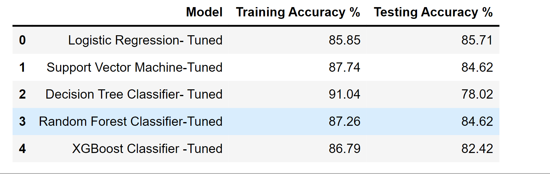
df_result_tuned

Output:

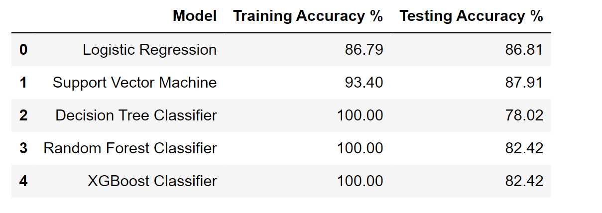
df_result

Output:

The outcomes don't appear to have significantly improved following hyperparameter adjustment. Maybe due to the tiny dataset.

According to Random Forest and XGBoost, the importance of the features

def feature_imp(df, model):
    fi = pd.DataFrame()
    fi["feature"] = df.columns
    fi["importance"] = model.feature_importances_
    return fi.sort_values(by="importance", ascending=False)


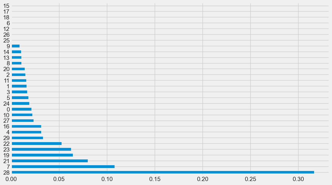
feature_imp(X, random_forest_clf).plot(kind='barh', figsize=(12,7), legend=False)

Output:

<AxesSubplot:>

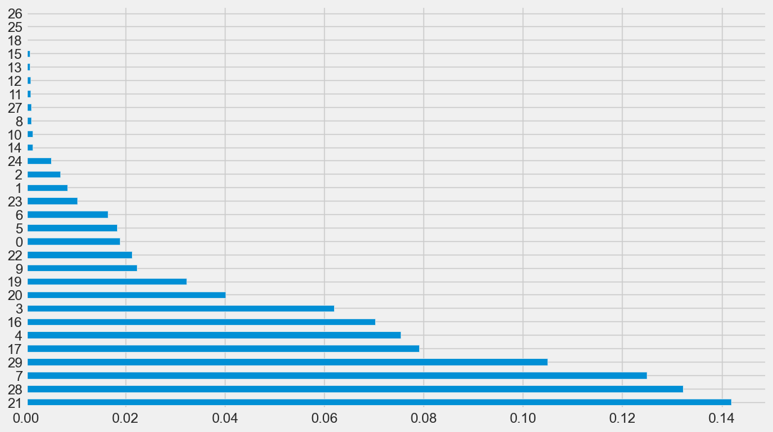
feature_imp(X, xgb_classifier).plot(kind='barh', figsize=(12,7), legend=False)

Output:

<AxesSubplot:>