Logistic Regression
The Logistic regression model is a supervised learning model which is used to forecast the possibility of a target variable. The dependent variable would have two classes, or we can say that it is binary coded as either 1 or 0, where 1 stands for the Yes and 0 stands for No.
It is one of the simplest algorithms in machine learning. It predicts P(Y=1) as a function of X. It can be used for various classification problems such as Diabetic detection, Cancer detection, and Spam detection.
Types of Logistic Regression
Logistic regression with binary target variables is termed as binary logistic regressions. The target variables can be categorized into two or more categories, which can be predicted. The logistic regression can be further classified into the following categories:
1. Binary: In this type of classification, the dependent variable will have either of the two cases; either 1 or 0, such that 1 represents win/yes and 0 is for loss/no.
- Multinomial: It is that kind of classification where a dependent variable can have three or even more unordered types with no significance. They denote Type-A, Type-B, and Type-C
- Ordinal: In this, the dependent variable can have three or more ordered types or the types with quantitative significance.
Assumptions in Logistic Regression
- In binary logistic regression, the target should be binary, and the result is denoted by the factor level 1.
- The independent variables should be independent of each other, in a sense that there should not be any multi-collinearity in the models.
- Only meaningful variables should be included in the model.
- For a logistic regression model, large sample size to be included
Binary Logistic Regression Model
It is one of the simpler logistic regression models in which the dependent variables are in two forms; either 1 or 0. It models a relationship between multiple predictor/independent variables and a binary dependent variable in order to discover the finest suitable model. It calculates the probability of an occurring event by the best-fitted data to the logit function. In this the linear function is used to feed as input to the other function, which is mathematically given as;
y = b0+b1x
Now apply the sigmoid function to the line;

Using the above two equations, we can deduce the logistic regression equation as follows;
ln = p/(1-p)=b0+b1x
We will see how the logistic regression manages to separate some categories and predict the outcome. For this, we will use a database which contains the information about the user in Social Network, such as User ID, Age, Gender, and Estimated Salary. The social_network has many clients who can put ads on a social network. One of the employees from Car Company has launched an SUV car on the ridiculously low price.
We are trying to see which users on the social network are going to buy the SUV on the basis of age & estimated salary variable. So, our matrix of the feature will be Age & Estimated Salary. We are going to find the correlation between them and also if they will purchase or not.
We will first undergo importing libraries as well as the dataset, and then we will perform data pre-processing steps;
#import the library and the dataset
import numpy as np
import pandas as pd
import matplotlib.pyplot as mpt
dataset= pd.read_csv ('Social_Network_Ads.csv')
After importing the data, you can check it by clicking on a dataset in Variable Explorer. This is the data given below:
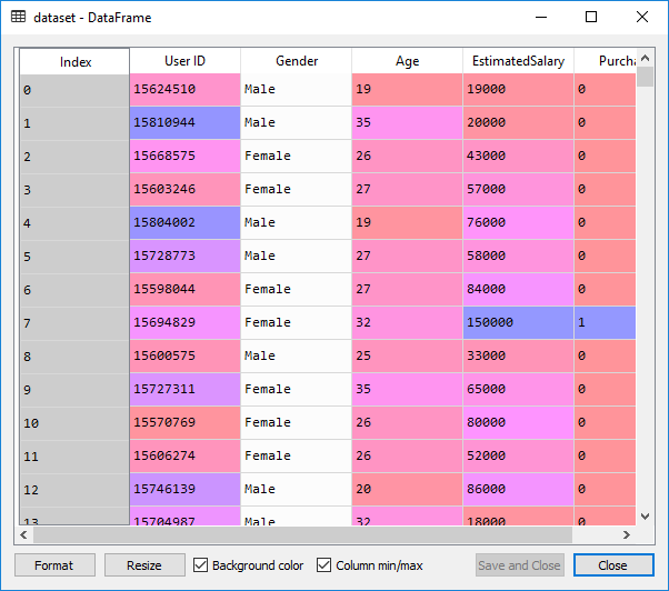
Now we will extract the feature matrix and the matrix of the dependent variable. The feature matrix is contained in the X variable, and the dependent variable matrix is retained in the Y variable.
#extracting matrix of independent variables and dependent variables
X= dataset.iloc [:,[2,3]]. values
Y= dataset.iloc [:, 4].values
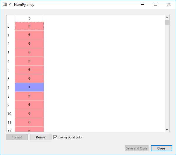
On executing the above two lines, the following output is given below:
For X:

For Y:
We will now split the dataset into a training set and the test set. As we have 400 observations, so a good test size would be 300 observations in the training set and the leftover 100 observations in the test set. And then we will apply feature scaling, as we want the accurate results to predict which users are actually going to buy the SUV’s.
#splitting the dataset
from sklearn. model_selection import train_test_split
X_train, X_test, Y_train, Y_test=train_test_split(X,Y,test_size=0.25,random_state=0)
#feature scaling
from sklearn.preprocessing import StandardScaler
sc_X=StandardScaler()
X_train=sc_X.fit_transform(X_train)
X_test=sc_X.transform(X_test)
Output:
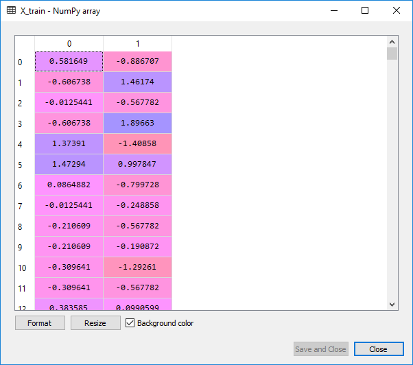
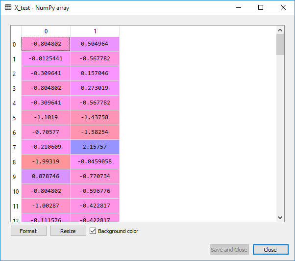
From the images given above, it can be clearly seen that the X_train and X_test are well scaled, but we have not scaled Y_train and Y_test as they consist of the categorical data.
Now that our data is well pre-processed, we are ready to build our Logistic Regression model. We will fit the Logistic regression to the training set. For this, we will first import the Linear model library because the logistic regression is the linear classifier. Since we are working here in 2D, our two categories of users will be separated by a straight line.
A new variable classifier will be created, which is a Logistic Regression object, and to create it a LogisticRegression class would be called. We will only include the random_state parameter to have the same results. And then we will take the classifier object and fit it to the training set using the fit() method, so that the classifier can learn the correlation between the X_train and the Y_train.
#fitting Logistic regression to the training set
from sklearn.linear_model import LogisticRegression
classifier = LogisticRegression(random_state=0)
classifier.fit(X_train, Y_train)
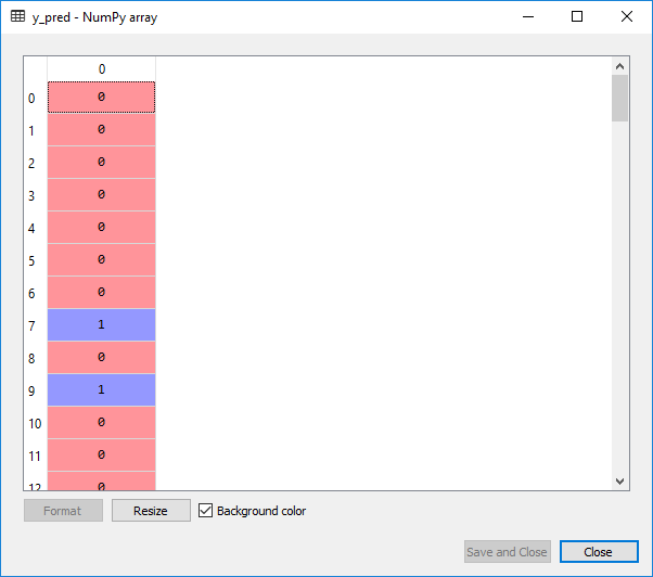
After learning the correlations, the classifier will now be able to predict the new observations. To test its predictive power, we will use the test set. A new variable y_pred will be introduced as it would going to be the vector of predictions. We will use predict() method of logistic regression class, and in that, we will pass the X_test argument.
#predicting the test set results
y_pred=classifier.predict(X_test)
Output:
This is the output we, get after implementation of the above line:
Now we will evaluate if our logistic regression model understood the correlations correctly in a training set to see how it will make the predictions on a new set or a test set. We will make a confusion matrix which will contain the correct predictions as well as the incorrect predictions made by our model.
So, for that, we will import a function from sklearn.metrics library. A new variable cm is then created, and we will pass some parameters such as; Y_test which is a vector of real values telling yes/no if the user really bought the car, Y_pred which is the vector of prediction,
from sklearn.metrics import confusion_matrix
cm=confusion_matrix(Y_test, y_pred)
Output:
array([[65,  3],
[ 8, 24]], dtype=int64)
From the above output, 65+24=89 are the correct predictions, whereas 3+8=11 are the incorrect ones.
Next, we will have a graphic visualization of our result in which we will clearly see a decision boundary of the classifier and the decision regions. We are going to make a graph so that we can clearly see the regions where logistic regression model predicts Yes in a case when the user is going to purchase the SUV and No when the user will not purchase the product.
To visualize the training set results, we will first import the ListedColormap class to colorize all the datapoints. Then we will create some local variables X_set and y_set to replace the X_train and Y_train. The command np.meshgrid will help us to create a grid with all the pixel points. We have taken the minimum age value to be -1, as we do not want out points to get squeezed and maximum value equals to 1, to get the range of those pixels we want to include in the frame and same we have done for the salary. We have taken the resolution equals to 0.01. We will then use the contour() to make contour between two prediction regions. After that we will use predict() of Logistic Regression classifier to predict which of the pixels points belong to 0 and 1. Then if the pixel point belong to o, it will be colourized as red or if it belong to 1, it will be colourized as green.
# Visualising the Training set results
from matplotlib.colors import ListedColormap
X_set, y_set = X_train, Y_train
X1, X2 = np.meshgrid(np.arange(start = X_set[:, 0].min() - 1, stop = X_set[:, 0].max() + 1, step  =0.01),
np.arange(start = X_set[:, 1].min() - 1, stop = X_set[:, 1].max() + 1, step = 0.01))
mpt.contourf(X1, X2, classifier.predict(np.array([X1.ravel(), X2.ravel()]).T).reshape(X1.shape),
alpha = 0.75, cmap = ListedColormap(('red', 'green')))
mpt.xlim(X1.min(), X1.max())
mpt.ylim(X2.min(), X2.max())
for i, j in enumerate(np.unique(y_set)):
mpt.scatter(X_set[y_set == j, 0], X_set[y_set == j, 1],
c = ListedColormap(('red', 'green'))(i), label = j)
mpt.title('Logistic Regression (Training set)')
mpt.xlabel('Age')
mpt.ylabel('Estimated Salary')
mpt.legend()
mpt.show()
Output:
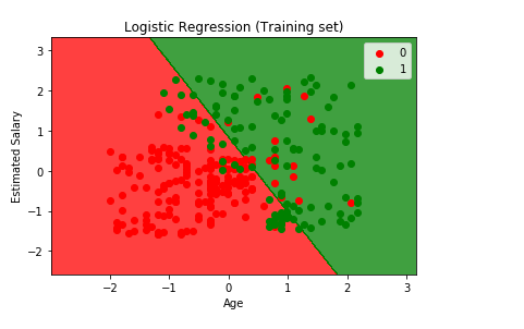
From the graph given above, we can see some red points and some green points. All these points are the observation points from the training set i.e. these were all the users of Social_Network which were selected to go to the training set. And each of these users are characterized by their age on X-axis and estimated salary on Y-axis.
The red points are the training set observations for which the dependent variable purchased is zero means the users who did not buy SUV, and for the green points the dependent variable purchased is equal to one are those users who actually bought SUV.
From the output given above, some of the following interpretations are made on the basis of the observations:
- We can see that the young people with low estimated salary is in the red region who didn’t buy the SUV as these are the real observation points, whereas in the green region there are older people with high estimated salary bought the SUV.
- Besides this, it can be seen that older people with low estimated salary actually bought the SUV.
- And on the other hand, we can see the young people with high estimated salary who bought the SUV.
Now the question arises that what is the goal of Classification? What are making the classifiers? What will they really do?
So, the goal is here to classify the right users into the right category which means we are trying to make a classifier which will successfully segregate right users into the right category and are represented by the prediction region. By prediction region, we meant the red region and the green region. For each user in the red region, the classifier predicts the users who dint buy the SUV, and for each user in the green region, it predicts the user who actually bought the SUV, such that the both these regions are separated by a straight line which is called as prediction boundary.
Here the prediction boundary is a straight line, and it means that our logistic regression classifier is a linear classifier. Since our logistic regression classifier is a linear classifier, so our prediction boundary will be the straight line and just a random one. Similarly, if we were in 3Dimension, then the prediction boundary would have been a straight plane separating two spaces. As it is a training set, our classifier successfully learned how to make the predictions based on this information.
Now we will see how out logistic regression classifier predicts the test set based on which our model wasn’t built and is carried out in the same way as done in the earlier step.
# Visualising the Test set results
from matplotlib.colors import ListedColormap
X_set, y_set = X_test, Y_test
X1, X2 = np.meshgrid(np.arange(start = X_set[:, 0].min() - 1, stop = X_set[:, 0].max() + 1, step  =0.01),
np.arange(start = X_set[:, 1].min() - 1, stop = X_set[:, 1].max() + 1, step = 0.01))
mpt.contourf(X1, X2, classifier.predict(np.array([X1.ravel(), X2.ravel()]).T).reshape(X1.shape),
alpha = 0.75, cmap = ListedColormap(('red', 'green')))
mpt.xlim(X1.min(), X1.max())
mpt.ylim(X2.min(), X2.max())
for i, j in enumerate(np.unique(y_set)):
mpt.scatter(X_set[y_set == j, 0], X_set[y_set == j, 1],
c = ListedColormap(('red', 'green'))(i), label = j)
mpt.title('Logistic Regression (Test set)')
mpt.xlabel('Age')
mpt.ylabel('Estimated Salary')
mpt.legend()
mpt.show()
Output:
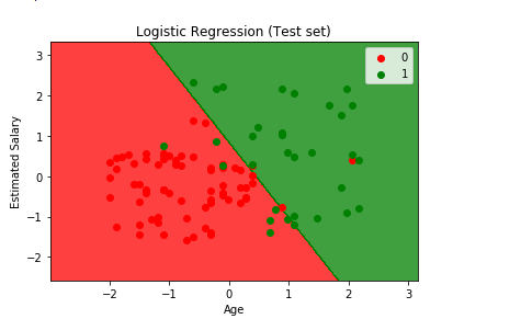
From the above output image, it can be seen that the prediction made by the classifier produces a good result and predicts really well as all the red points are in the red region, but only a few green points are there in the red region which is acceptable not a big issue. This is due to the 11 incorrect predictions which we saw in the confusion matrix and can be counted from here too by calculation the red and green points present in the alternate regions. It can be seen that in the red region, red points indicate the people who did not buy the SUV and in the green region the people who bought the SUV.