Hierarchical Clustering Algorithm
Introduction to Hierarchical Clustering
The other unsupervised learning-based algorithm used to assemble unlabeled samples based on some similarity is the Hierarchical Clustering. There are two types of hierarchical clustering algorithm:
1. Agglomerative Hierarchical Clustering Algorithm
It is a bottom-up approach. It does not determine no of clusters at the start. It handles every single data sample as a cluster, followed by merging them using a bottom-up approach. In this, the hierarchy is portrayed as a tree structure or dendrogram.
2. Divisive Hierarchical Clustering Algorithm
In this approach, all the data points are served as a single big cluster. It is a top-down approach. It starts with dividing a big cluster into no of small clusters.
Working of Agglomerative Hierarchical Clustering Algorithm:
Following steps are given below, that demonstrates the working of the algorithm;
Step 1: We will treat each data point as an individual cluster, and for that, let us assume m no of datapoints to be there, such that m no of clusters also exist.
Step 2: In the next step, we will construct one big cluster by merging the two neighboring clusters. It will lead to m-1 clusters.
Step 3: We will merge more clusters to form a bigger cluster that will result in m-2 clusters.
Step 4: We will reiterate the previous three steps to form the biggest cluster until m turns out to be 0 (when no more data samples are left to be joined).
Step 5: Once the biggest cluster is formed, we will incorporate dendrograms to split it into multiple clusters on the basis of the problem.
Implementation in Python
As we already know, the mall dataset consists of the customer’s information who have subscribed to the membership card and the ones who frequently visits the mall. The mall allotted CustomerId to each of the customers. Also, at the time of subscription, the customer provided their personal details to the mall, which made it easy for the mall to compute the SpendingScore for each customer based on several benchmarks.
The values taken by the SpendingScore is in between 1 to 100. The closer the spending score is to 1, the lesser is the customer spent, and the closer the spending score to 100 more is the customer spent. It is done to segment the customers into different groups easily. But the only problem is that the mall has no idea what these groups might be or even how many groups are they looking for. So, this is the same problem that we faced while doing k-means clustering, but now here we will solve it with a hierarchical clustering algorithm.
We will start with importing the libraries and the same dataset that we used in the K-means clustering algorithm. Next, we will select the columns of our interest i.e., Annual Income and Spending Score.
 # Import the libraries
 import numpy as np
 import matplotlib.pyplot as plt
 import pandas as pd
 # Import the dataset
 dataset = pd.read_csv('Mall_Customers.csv')
 X = dataset.iloc[:, [3, 4]].values
In the previous algorithm, after importing the libraries and the dataset, we used the elbow method, but here we will involve the concept of the dendrogram to find the optimal no of clusters. For this, we will first import an open-source python scipy library (scipy.cluster.hierarchy) named as sch. It contains the tool for hierarchical clustering and building the dendrograms.
We will start by creating a variable called dendrogram, which is actually an object of sch. We will pass sch.linkage as an argument where linkage is an algorithm of hierarchical clustering. In linkage, we will specify the data i.e., X on which we are applying and the method that is used to find the cluster. Here we are using the ward method. It actually minimized the variance in the cluster.
In the previous K-means clustering algorithm, we were minimizing the within-cluster sum of squares to plot the elbow method, but here it is almost the same, the only difference is that here we are minimizing the within cluster variants. Unlike the K-means, we are not required to implement for loop here, just implementing this one line code, we are able to build the dendrogram. We have titled our plot as Dendrogram, xlabel as Customers, and ylabel as Euclidean distances because the vertical lines in the dendrogram are the distances between the centroids of the clusters.
# Using the dendrogram to find the optimal number of clusters
import scipy.cluster.hierarchy as sch
dendrogram = sch.dendrogram(sch.linkage(X, method = 'ward'))
plt.title('Dendrogram')
plt.xlabel('Customers')
plt.ylabel('Euclidean distances')
plt.show()
Output:
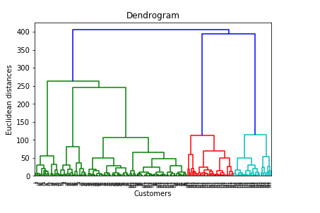
Here at the bottom, we are having all our customers, and vertical lines on this dendrogram represent the Euclidean distances between the clusters. And this dendrogram represents all the different clusters that were found during the hierarchical clustering process. Now to find the optimal no of clusters, we will look for the largest vertical distance without crossing the horizontal line and count the vertical lines in the space here i.e., five, which is the exact same result that we obtained with K-means elbow method.
After finding the optimal no. of the cluster, our next step is to fit the hierarchical clustering to the dataset. We will start by importing the AgglomerativeClustering class from the scikit learn. Then we will create an object hc of class AgglomerativeClustering and will some of the following parameters:
- The first parameter is n_cluster i.e., the no of clusters that we already know is equal to 5.
- The second parameter that we will pass is the affinity, which is the distance that does the linkage. So, here we are using the Euclidean.
- The last and the most important parameter is the linkage, the same one that we used while building the dendrogram, which is a ward method that tries to minimize the variance in each of the clusters.
# Fit the Hierarchical Clustering to the dataset
from sklearn.cluster import AgglomerativeClustering
hc = AgglomerativeClustering(n_clusters = 5, affinity = 'euclidean', linkage = 'ward')
By now, we are done with preparing hierarchical clustering, now we will fit the hierarchical clustering to the data X while creating the clusters vector y_hc that tells for each customer which cluster the customer belongs to. The agglomerative clustering class also contains fit_predict(), which is going to return the vector of clusters. So, we have used fit_predict(X) to specify that we are fitting the agglomerative clustering algorithm to our data X and also predicting the clusters of customers of data X. Basically, we did exactly the same as the K-means clustering, the only difference is the class (i.e., the agglomerative class) we have used here.
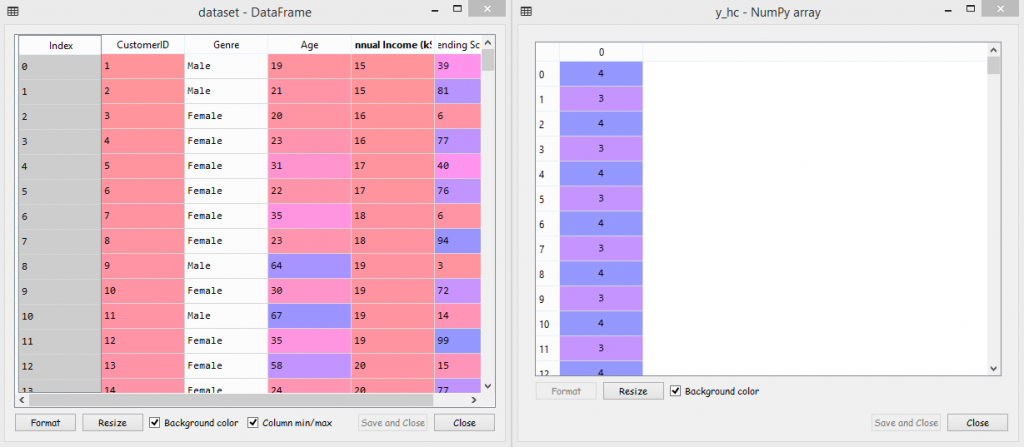
y_hc = hc.fit_predict(X)
On executing it, we will see that at variable explorer, a new variable y_hc has been created. And on comparing our dataset with y_hc, we will see CustomerId no. 1 belongs to cluster 4, CustomerId 44 belongs to cluster 1, and so on. So we did a good job by correctly fitting the hierarchical clustering algorithm to our data X.
Output:
Now we will visualize the clusters of customers. In this section we will use exactly the same code that we used in the K-means clustering algorithm for visualizing the clusters, the only difference is the vectors of clusters i.e. y_hc will be used here for hierarchical clustering instead of y_kmeans that we used in the previous model which means we will replace y_kmeans by y_hc. Also we will discard the last line from our code that we used to plot the clusters centroid in k-means algorithm, as here it is not required. And then we will execute the code.
# Visualize the clusters
plt.scatter(X[y_hc == 0, 0], X[y_hc == 0, 1], s = 100, c = 'red', label = 'Cluster 1')
plt.scatter(X[y_hc == 1, 0], X[y_hc == 1, 1], s = 100, c = 'blue', label = 'Cluster 2')
plt.scatter(X[y_hc == 2, 0], X[y_hc == 2, 1], s = 100, c = 'green', label = 'Cluster 3')
plt.scatter(X[y_hc == 3, 0], X[y_hc == 3, 1], s = 100, c = 'cyan', label = 'Cluster 4')
plt.scatter(X[y_hc == 4, 0], X[y_hc == 4, 1], s = 100, c = 'magenta', label = 'Cluster 5')
plt.title('Clusters of customers')
plt.xlabel('Annual Income (k$)')
plt.ylabel('Spending Score (1-100)')
plt.legend()
plt.show()
Output:
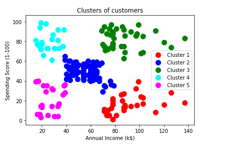
From the above output image, it can be seen that the 1st cluster is the red cluster and customers in this cluster have high income and low spending score named as careful customers, the 2nd cluster is the blue one present in the middle contains the customers with average income and average spending score called as standard customers, then the 3rd cluster is the green cluster with customers having high income and high spending score termed as target of the marketing campaigns, 4th cluster is the one on the upper left corner containing the customers with low income high spending score labelled as careless customers, and the last one is 5th cluster that comprises of low income and low spending score customers called as the sensible.
So, here we complete our hierarchical clustering algorithm. You can use the same code for any other business problem with a different database, keeping one thing that the last section is only applicable for clustering in 2D. In that, you will be needed to change the higher dimension 2D and then execute it.