Data Preprocessing in Machine Learning

Before starting a machine learning project, data is an essential thing needed before starting a project. The data used in ML projects is in CSV (Comma Separated Value) format. It is the most common as well as simple format formats of data used in ML projects, as it is used to save the tabular data or spreadsheets in a plain text.  

A CSV file consists of a header file for each field containing the information in it, separated by the same type of delimiter for both header file and data file. The header file states how to interpret the data file.

• Case 1: - Data file containing a header file:- If the data file contains a header file, then it will automatically allocate names to each of the columns.

Following are some cases regarding header file that should be taken in account: -

• Case 2: - Data file not containing a header file: -  In this case, we need to manually assign the names to each column in the data file. 

It is required to specify explicitly if your CSV file contains a header file or not.

Comments: - There is a significance of comments present in the data file. It is denoted by (#) written at the starting of the line.

Delimiters: - In the CSV file (,) comma character is the standard delimiter. The main role of the delimiter is to isolate the values in the data file. Apart from this, there are many other delimiters that can be used such as a tab or whitespace, so it can be said that they play a key role while uploading a data into the ML projects. They need to be specified in case of using a different delimiter other than the standard one.

Quotes: - Here, the double quotation marks (“”) is the standard quote character. In case you want to use a different quote than you need to specify them explicitly. 

Importing the Libraries

Before we move on to data pre-processing, we first need to import some of the predefined python libraries. Here we are going to use some of the standard python libraries such as; NumPy, Pandas, Matplotlib.

NumPy

NumPy stands for Numerical Python. It is a python library which enables a programmer to implement linear operations, mathematical as well as logical operations on arrays, Fourier transforms and routine to manipulate the shapes.

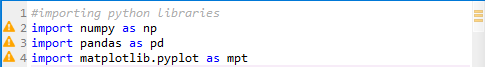
import numpy as np

Pandas

Pandas in as open-source python library. It provides high-performance data manipulation and analyzing tool. It is commonly used for data handling and analysis.

import pandas as pd

Matplotlib

An open-source library which is used to plot the charts in the python. It is basically used to visualize the data. It is necessary to import a sub-library called pyplot.

import matplotlib.pyplot as mpt

An image is given below which shows how to import the python libraries;

As Pandas is the best library, so now we will see how to import the data file from the current working directory using Pandas. To read a CSV file we are using read_csv() function. It is used to read a CSV files both locally or from a URL.

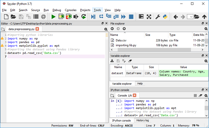
Here dataset is the name of a variable which is used to store the data. In the read_csv() function we have passed the name of the dataset which we are going to use. Once the code is executed successfully, the data will get uploaded in the code.

To check the dataset, you may click on Variable explorer and select dataset as given below in the image. 

Extraction of dependent and independent variables

It is very necessary to distinguish between the dependent as well as the independent variables. Here in our chosen dataset, the independent variables are the Country, Age, Salary, and the dependent variable is the Purchased.

Extraction of Independent variable

To extract the independent variables from the given dataset, we will use iloc[ ] method of pandas library.

X= dataset.iloc [: , : -1]. values

Here the first (:)is used to indicate all rows, whereas the second (:) is used for all the columns. We have used -1 as we do not want to consider the last column of the dataset as it contains the dependent variable, which will help us in extracting the feature matrix.

Output:

array([['France', 44.0, 72000.0],
['Spain', 27.0, 48000.0],
['Germany', 30.0, 54000.0],
['Spain', 38.0, 61000.0],
['Germany', 40.0, nan],
['France', 35.0, 58000.0],
['Spain', nan, 52000.0],
['France', 48.0, 79000.0],
['Germany', 50.0, 83000.0],
['France', 37.0, 67000.0]], dtype=object) 

Here you can see the three first column of the dataset from the output given above.

Extraction of a Dependent Variable

Again we will use Pandas iloc[] method to extract the dependent variable.

Y= dataset.iloc [: , 3].values

Here it indicate all the lines of last column. It will output an array of dependent variables.

Output:

array(['No', 'Yes', 'No', 'No', 'Yes', 'Yes', 'No', 'Yes', 'No', 'Yes'],
dtype=object) 

Preparing the Data

Now the next step is preparing our data so that our machine learning model runs correctly. While working on a dataset, there may be a case where the data is missing. So, in that case, we have to handle the problem in such a way so that the machine learning model can run correctly.

Different ways to handle missing data

Data can be handle in two ways:

1) By deleting specific row/ column

This approach is usually used in the case of null values. In this, a particular row or a column containing null value is deleted. As this is not an efficient way to handle a missing, it may cause loss of important data.

2.) By calculating the mean value

It calculates the mean value of that particular row/column where the value is missing and replaces the missing value. It is useful for the features containing the numeric data like age, salary, year, etc.

So, to calculate the mean value, we are using Scikit-learn pre-processing library. An example is given below, in which we have used Imputer class.

from sklearn.preprocessing import Imputer
imputer=Imputer(missing_values='NaN',strategy='mean',axis=0)
imputer=imputer.fit(X[:, 1:3])
X[:,1:3]=imputer.transform(X[:, 1:3]) 

Output:

array([['France', 44.0, 72000.0],
['Spain', 27.0, 48000.0],
['Germany', 30.0, 54000.0],
['Spain', 38.0, 61000.0],
['Germany', 40.0, 63777.77777777778],
['France', 35.0, 58000.0],
['Spain', 38.77777777777778, 52000.0],
['France', 48.0, 79000.0],
['Germany', 50.0, 83000.0],
['France', 37.0, 67000.0]], dtype=object) 

From the output given above, it can be seen that the missing values has been replaced with the mean of the rest column.

Encoding categorical data

A data having some specific category is called as categorical data. In our dataset, we have two categorical data, i.e., country and purchased.  

Since machine learning is based on mathematical equations, so it will cause a problem if we keep the text on categorical variables in the equations because we only want numbers. That’s why we need to encode text of the categorical variable into the nos.

from sklearn.preprocessing import LabelEncoder
labelencoder_X=LabelEncoder()
X[:,0]=labelencoder_X.fit_transform(X[:,0]) 

Output:

array([[0, 44.0, 72000.0],
[2, 27.0, 48000.0],
[1, 30.0, 54000.0],
[2, 38.0, 61000.0],
[1, 40.0, 63777.77777777778],
[0, 35.0, 58000.0],
[2, 38.77777777777778, 52000.0],
[0, 48.0, 79000.0],
[1, 50.0, 83000.0],
[0, 37.0, 67000.0]], dtype=object) 

For encoding text into numerical no. we have imported LabelEncoder() which is a class of sklearn library. Since we have three country variables which are now encoded into 0, 1, and 2, machine learning model may believe in the fact that these variables are having some relation in between them, which may produce an incorrect output. So, to resolve this issue dummy variables are used.

Dummy Variables

Dummy variables are those variables which have either of the values 0 or 1. The value 1 depicts the presence of any variable in a particular column, elsewhere 0 is for the absence.

As our dataset consists of three categories, so there will be three columns containing 1 and 0.  OneHotEncoder class of pre-processing library.

For Independent Variables

from sklearn.preprocessing import LabelEncoder, OneHotEncoder 
labelencoder_X=LabelEncoder()
X[:,0]=labelencoder_X.fit_transform(X[:,0])
onehotencoder=OneHotEncoder(categorical_features=[0])
X=onehotencoder.fit_transform(X).toarray() 

Output:

array([[0.00000000e+00, 1.00000000e+00, 0.00000000e+00, 0.00000000e+00,
4.40000000e+01, 7.20000000e+04],
[1.00000000e+00, 0.00000000e+00, 0.00000000e+00, 1.00000000e+00,
2.70000000e+01, 4.80000000e+04],
[1.00000000e+00, 0.00000000e+00, 1.00000000e+00, 0.00000000e+00,
3.00000000e+01, 5.40000000e+04],
[1.00000000e+00, 0.00000000e+00, 0.00000000e+00, 1.00000000e+00,
3.80000000e+01, 6.10000000e+04],
[1.00000000e+00, 0.00000000e+00, 1.00000000e+00, 0.00000000e+00,
4.00000000e+01, 6.37777778e+04],
[0.00000000e+00, 1.00000000e+00, 0.00000000e+00, 0.00000000e+00,
3.50000000e+01, 5.80000000e+04],
[1.00000000e+00, 0.00000000e+00, 0.00000000e+00, 1.00000000e+00,
3.87777778e+01, 5.20000000e+04],
[0.00000000e+00, 1.00000000e+00, 0.00000000e+00, 0.00000000e+00,
4.80000000e+01, 7.90000000e+04],
[1.00000000e+00, 0.00000000e+00, 1.00000000e+00, 0.00000000e+00,
5.00000000e+01, 8.30000000e+04],
[0.00000000e+00, 1.00000000e+00, 0.00000000e+00, 0.00000000e+00,
3.70000000e+01, 6.70000000e+04]]) 

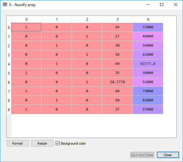
It can be seen from the output given above, that all the variables have been encoded into 0 and 1. For a more clear view, it can be seen by clicking on X in Variable Explorer pane. The output will be as shown in the image given below:

For Dependent Variable

labelencoder_Y=LabelEncoder()
Y=labelencoder_Y.fit_transform(Y) 

Here, in this case, we will only use the object labelencoder of class LabelEncoder. We have not used the class OneHotEncoder as our dependent variable does not contain more than two absolute value so that it will be automatically encoded into either 1 or 0.

Output:

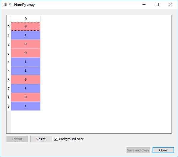
array([0, 1, 0, 0, 1, 1, 0, 1, 0, 1])

It can be seen the same way as we did in the earlier step, but now we will have to click on Y in Variable Explorer pane as shown in the image given below:

Splitting the Dataset into the Training set and Test set

In machine learning pre-processing, we prepare the data for the model by splitting the dataset into the test set and training set. It is one of the significant step used for enhancing the performance of the machine learning model.

As the model is going to learn from the data to make the predictions. Imagine, if the dataset is trained on some specific dataset and is tested on some different dataset. Then, in that case, the performance will get degraded because it will create difficulty for the model to understand the different correlations.

If we train the model in such a way that its training accuracy is very high, but we test it on a slightly different dataset, then, in that case, the performance will be decreased. So, in order to achieve better performance with a machine learning model, we try to deploy a model that will perform better with both training set as well as the test set.

A dataset can be defined as:

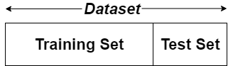
A Training set is a subset of a dataset and is used to train the model and here the output is already known, whereas a test set is also a subset of the dataset but is used to test the machine learning model on a dataset to predict an output.

from sklearn. model_selection import train_test_split
X_train, X_test, Y_train, Y_test=train_test_split(X,Y,test_size=0.2,random_state=0) 

From the code given above, the fundamental explanation is given below:

To split the database into a random train subset and test subset, we have incorporated train_test_split, which is a class of sklearn. Then we have used four variables, namely X_train, X_test, Y_train, and Y_test, to get the following outputs:

To split the database into a random train subset and test subset, we have incorporated train_test_split, which is a class of sklearn. Then we have used four variables, namely X_train, X_test, Y_train, and Y_test, to get the following outputs:

• X_train: independent variables for the training set
• X_test: independent variables for test set
• Y_train: dependent variables for the training set
• Y_test: dependent variables for test set

We have passed four input parameters in train_test_split() function, out of which first two are for the arrays of the data and the test_size is used to specify the size of the test set so as to divide the dataset into a training set and the test set. The test_size can be 0.5, 0.3, and 0.2 depending upon the requirement.

The random_state is used to set a seed for a random generator to always get the same result. Mostly random_state is set to 42. Upon the execution of the code the output is as given below:

Output:

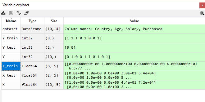
From the image given above, it can be clearly seen that the X and Y variables are divided into four different variables and can be checked by clicking on them in Variable explorer pane.

Feature Scaling

It is the last step in the pre-processing data phase. It is the way of equalizing the independent variables to a particular range. It is done in such a manner that all the variables are set to the same range and same scale so that no variable overshadow the other variable.

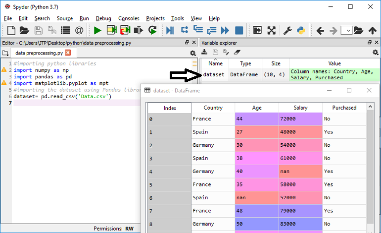
Consider the dataset given below:

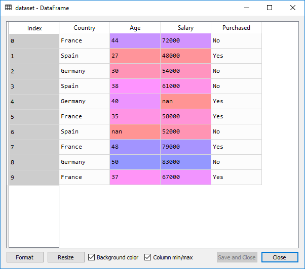
From the given image, it can be observed that the age and salary column, as they contain the numerical values. You can see that the variables are not on the same scale. The age is ranging from 27 to 50, and salary is ranging from 40k to 90k. As they have distinct scales, it may cause a problem in machine learning models because machine learning models are based on Euclidean Distances.

Since salary has a much higher range as that of the age, so the Euclidean distance would be dominated by the salary, that’s why we will transform the variables so that they can have values in the same scale. And for that feature scaling is performed.

We will import StandardScaler class of sklearn.preprocessing library.An object of StandardScaler class is created for independent variables, with the help of which we will fit and transform the training set.

from sklearn.preprocessing import StandardScaler
sc_X=StandardScaler()
X_train=sc_X.fit_transform(X_train)
X_test=sc_X.transform(X_test) 

For the test set, we will only perform transform(), as fit_transform() is already implemented in training set.

X_test=sc_X.transform(X_test)

Output:

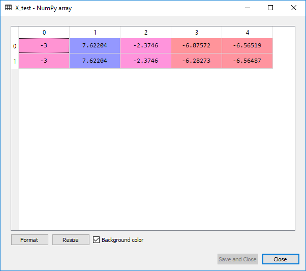
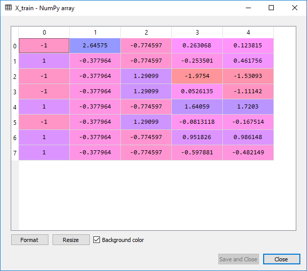
Upon the execution of above code, we will get following scaled values for the X_train and X_test:

X_train:

X_test: