Rainfall Prediction Using Machine Learning
Rainfall prediction using machine learning is an important topic that has gained a lot of attention in recent years. With climate change causing an increase in the severity and frequency of extreme weather events, accurate and reliable rainfall predictions are crucial for managing water resources and mitigating flood risks. In this article, we will discuss the various machine-learning techniques that are currently being used for rainfall prediction and their effectiveness.

One of the most widely used machine learning techniques for rainfall prediction is artificial neural networks (ANNs). ANNs are based on the structure of the human brain and are capable of learning and generalizing from data. They can be used to model complex non-linear relationships between rainfall and various atmospheric variables, such as temperature, humidity, and wind speed. One of the advantages of ANNs is that they can handle a large amount of input data, making them suitable for handling large-scale weather data.
Another popular machine-learning technique for rainfall prediction is the support vector machine (SVM). SVM is a supervised learning algorithm that is used for classification and regression tasks. It can be used to model the relationship between rainfall and various atmospheric variables and make predictions about future rainfall. One of the advantages of SVM is that it is able to handle high-dimensional data and has good generalization ability.
A third machine-learning technique that is commonly used for rainfall prediction is the decision tree. Decision trees are a non-parametric method, and they can handle both numerical and categorical data. It creates a tree-like model of decisions and their possible consequences, including the prediction of a target value. A decision tree can be used to find the most important variables that affect rainfall and make predictions about future rainfall.
Additionally, there are more advanced Machine Learning algorithms such as Random Forest, Gradient Boosting, etc. These are ensemble methods, which are constructed by combining multiple decision trees to improve the accuracy of predictions. These models are more robust and generalizable.
One of the most challenging aspects of using machine learning for rainfall prediction is the lack of high-quality data. Weather data can be noisy and incomplete, and it can be difficult to obtain accurate measurements of rainfall in certain areas. Additionally, many machine learning algorithms require a large amount of data to be trained and tested, which can be a problem in regions where data is scarce.
Challenges
In general, predicting rainfall can be a challenging task due to the complex and non-linear nature of the weather system. Machine learning models, such as random forest, gradient boosting, and long short-term memory (LSTM) networks, have been used for rainfall prediction with varying levels of success.
It's also important to consider the data quality and features used for the prediction, as well as the evaluation metric used to measure the performance of the model. A good practice would be to compare the model's predictions with the actual rainfall data and evaluate the model's performance using metrics such as mean absolute error (MAE), root means squared error (RMSE), and correlation coefficient (R-squared).
Now for reference, we will use ANN for the rainfall prediction on the dataset 'weatherAUS.csv'.We will try to predict the rainfall through the underlying code.
Rainfall Prediction Using Python
Importing Libraries
import numpy as np
import pandas as pd
import matplotlib.pyplot as plt
import seaborn as sns
import datetime
from sklearn.preprocessing import LabelEncoder
from sklearn import preprocessing
from sklearn.preprocessing import StandardScaler
from sklearn.model_selection import train_test_split
import seaborn as sns
from keras.layers import Dense, BatchNormalization, Dropout, LSTM
from keras.models import Sequential
from keras.utils import to_categorical
from keras.optimizers import Adam
from tensorflow.keras import regularizers
from sklearn.metrics import precision_score, recall_score, confusion_matrix, classification_report, accuracy_score, f1_score
from keras import callbacks


np.random.seed(0)
Loading Data
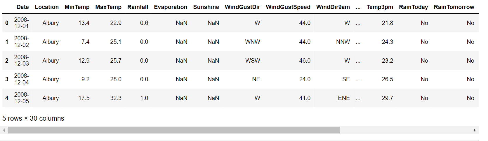
main_data = pd.read_csv("weatherAUS.csv")
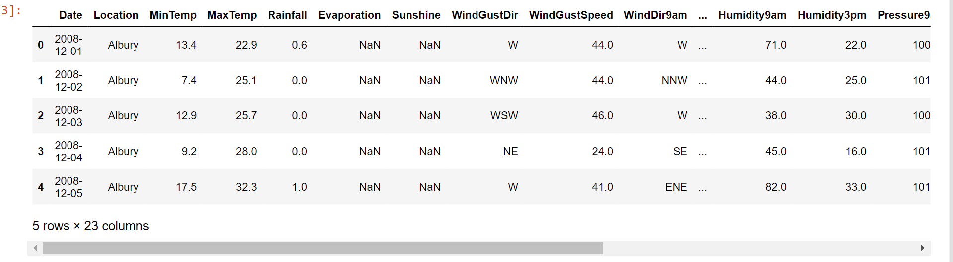
main_data.head()
Output:
Dataset Description
About ten years' worth of daily weather measurements from various points across Australia are included in the dataset. Several weather stations were used to gather observations.
We will utilize this information in our project to make predictions about whether it will rain the next day. The goal variable "RainTomorrow," which indicates whether or not it will rain the next day, is one of the 23 qualities.
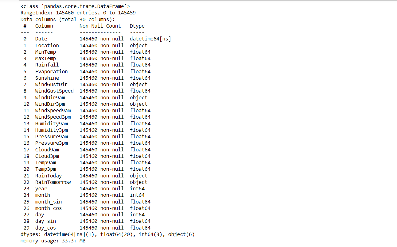
main_data.info()
Output:
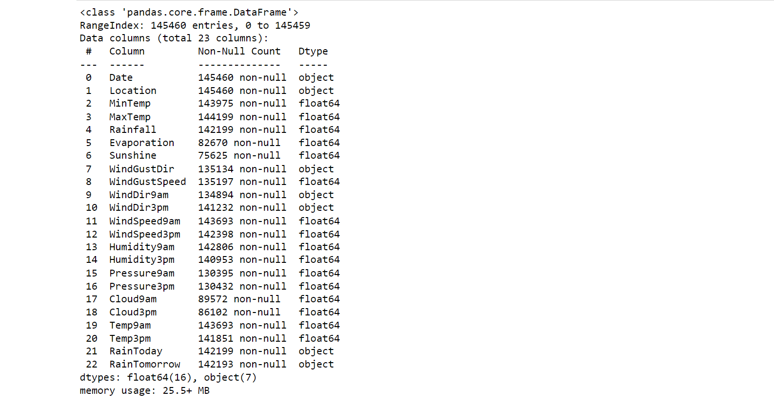
Here, we notice two things that are:
- The dataset has some missing values.
- The dataset has numeric and categorical values.
Data Visualisation
Data visualization can be an important tool in machine learning for predicting rainfall. By creating visual representations of the data, such as graphs and charts, it can be easier to identify patterns and trends in the data. These patterns and trends can then be used to train a machine-learning model to make predictions about future rainfall.
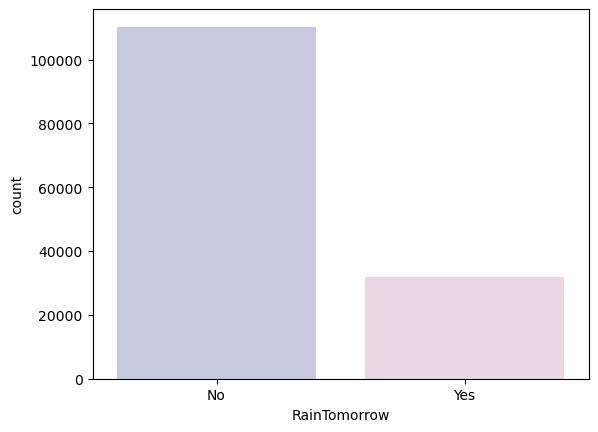
# Let's first evaluate the goal and check to see if our data is balanced.
col= ["#C2C4E2","#EED4E5"]
sns.countplot(x= main_data["RainTomorrow"], palette= col)
Output:
<AxesSubplot:xlabel='RainTomorrow', ylabel='count'>
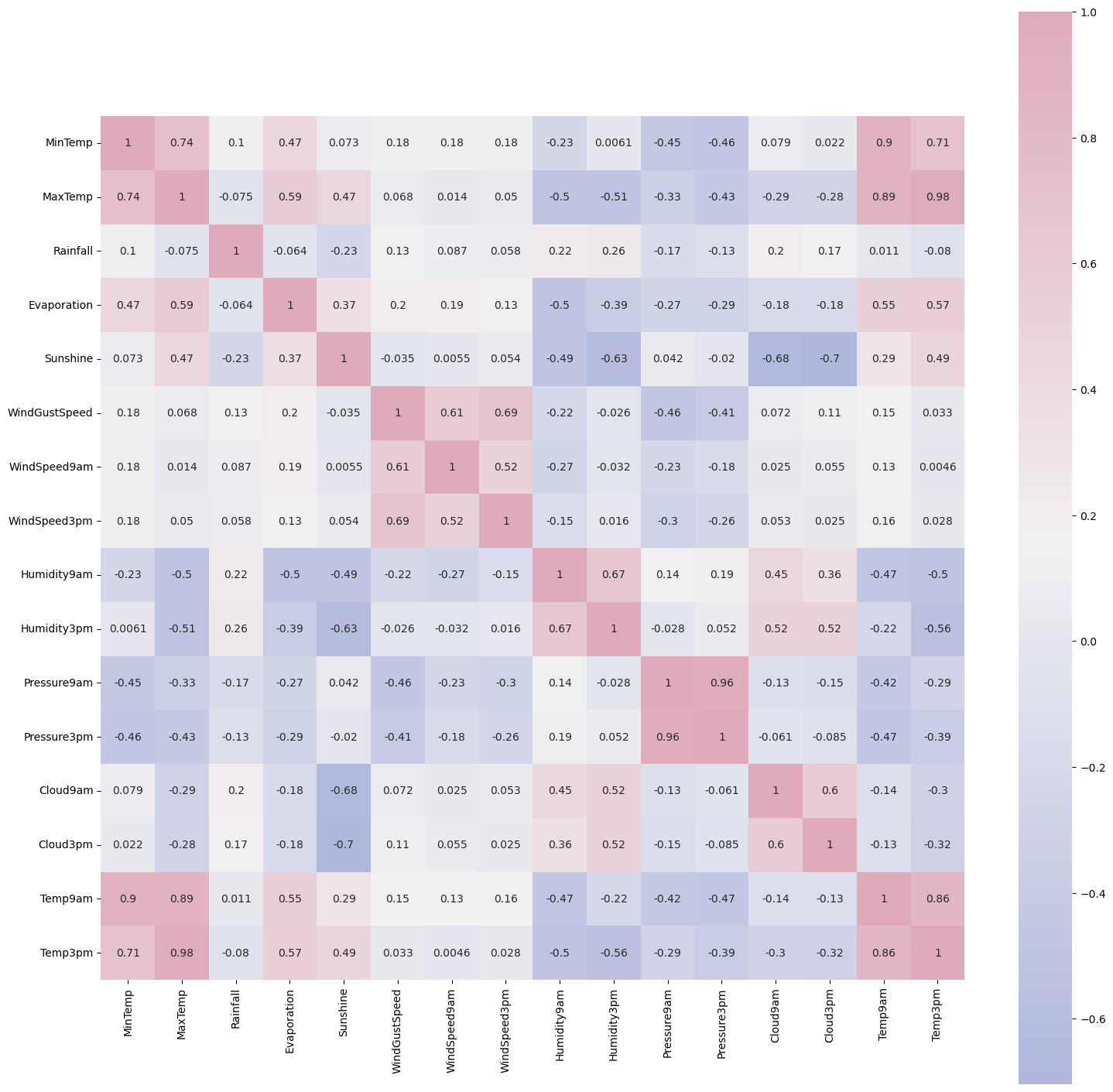
# Correlation (Numeric)
corrmatrix = main_data.corr()
cmap = sns.diverging_palette(260,-10,s=50, l=75, n=6, as_cmap=True)
plt.subplots(figsize=(18,18))
sns.heatmap(corrmatrix,cmap= cmap,annot=True, square=True)
Output:
<AxesSubplot:>
Parse Date into datetime
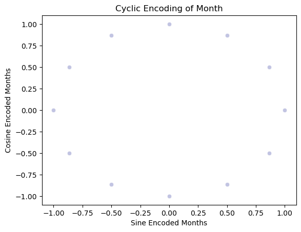
Our objective is to create a synthetic neural network (ANN). We will properly encode dates; our preference is to use a cyclic continuous feature that includes the months and days. Time and date are cyclical by nature. We divided the feature into periodic subsections to signal to the ANN model that the feature is cyclical. Months, days, and years, respectively. Now, we make two new features for each subsection by deriving a sine transform and a cosine transform from the subsection feature.
length_of_it = main_data["Date"].str.len()
length_of_it.value_counts()
Output:

# Since dates don't seem to have any faults, it is possible to convert data into datetime.
main_data['Date']= pd.to_datetime(main_data["Date"])
# establishing a year column
main_data['year'] = main_data.Date.dt.year


#  datetime cyclic parameter encoding function.
#  We favor months and days in a cyclic continuous feature since we intend to use this data in a neural network.
def encode(data_, col_, max_val):
    data_[col_ + '_sin'] = np.sin(2 * np.pi * data_[col_]/max_val)
    data_[col_ + '_cos'] = np.cos(2 * np.pi * data_[col_]/max_val)
    return data_


main_data['month'] = main_data.Date.dt.month
main_data = encode(main_data, 'month', 12)


main_data['day'] = main_data.Date.dt.day
main_data = encode(main_data, 'day', 31)


main_data.head()
Output:
section = main_data[:360]
tmi = section["day"].plot(color="#C2C4E2")
tmi.set_title("Distribution Of Days Over Year")
tmi.set_ylabel("Days In month")
tmi.set_xlabel("Days In Year")
Output:
Text(0.5, 0, 'Days In Year')
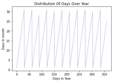
The data's "year" property repeats as predicted. However, this does not reflect the full cyclic nature in a continuous way. The continuous cyclical characteristic may be obtained by dividing the months and days into sine and cosine combinations. This can serve as an ANN's input features.
month_cyclic = sns.scatterplot(x="month_sin",y="month_cos",data=main_data, color="#C2C4E2")
month_cyclic.set_title("Cyclic Month Encoding")
month_cyclic.set_ylabel("Cosine Encoded Months")
month_cyclic.set_xlabel("Sine Encoded Months")
Output:
Text(0.5, 0, 'Sine Encoded Months')
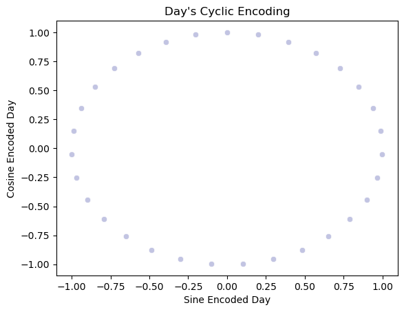
day_cyclic= sns.scatterplot(x='day_sin',y='day_cos',data=main_data, color="#C2C4E2")
day_cyclic.set_title("Day's Cyclic Encoding")
day_cyclic.set_ylabel("Cosine Encoded Day")
day_cyclic.set_xlabel("Sine Encoded Day")
Output:
Text(0.5, 0, 'Sine Encoded Day')
Now, We have to deal with the missing values in numerical and categorical variables separately.
Categorical Variables
# Obtaining a list of the category variables
# In the case of missing values in categorical, we use the mode of the column value to fill the missing space.
cat_lit = (main_data.dtypes == "object")
object_col = list(cat_lit[cat_lit].index)


print("Categorical variables:")
print(object_col)
Output:

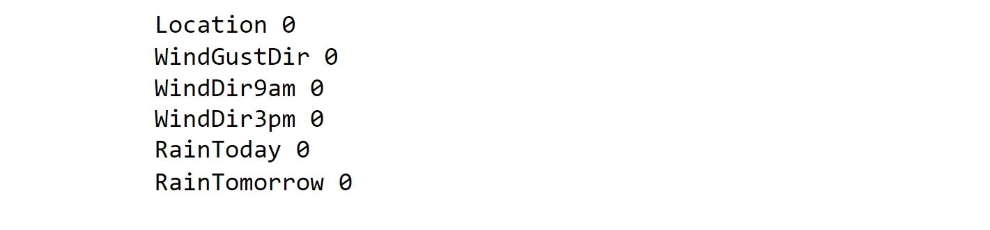
# values in category variables that are missing


for i in object_col:
    print(i, main_data[i].isnull().sum())
Output:
# using the mode of the column in value to fill in missing data
for i in object_col:
    main_data[i].fillna(main_data[i].mode()[0], inplace=True)
Numerical Variables
# Obtaining a list of numerical variables.
# # In the case of missing values in numerical value, we use the median of the column value to fill the missing space.
num_lit = (main_data.dtypes == "float64")
num_col = list(num_lit[num_lit].index)


print("Neumeric variables:")
print(num_col)
Output:

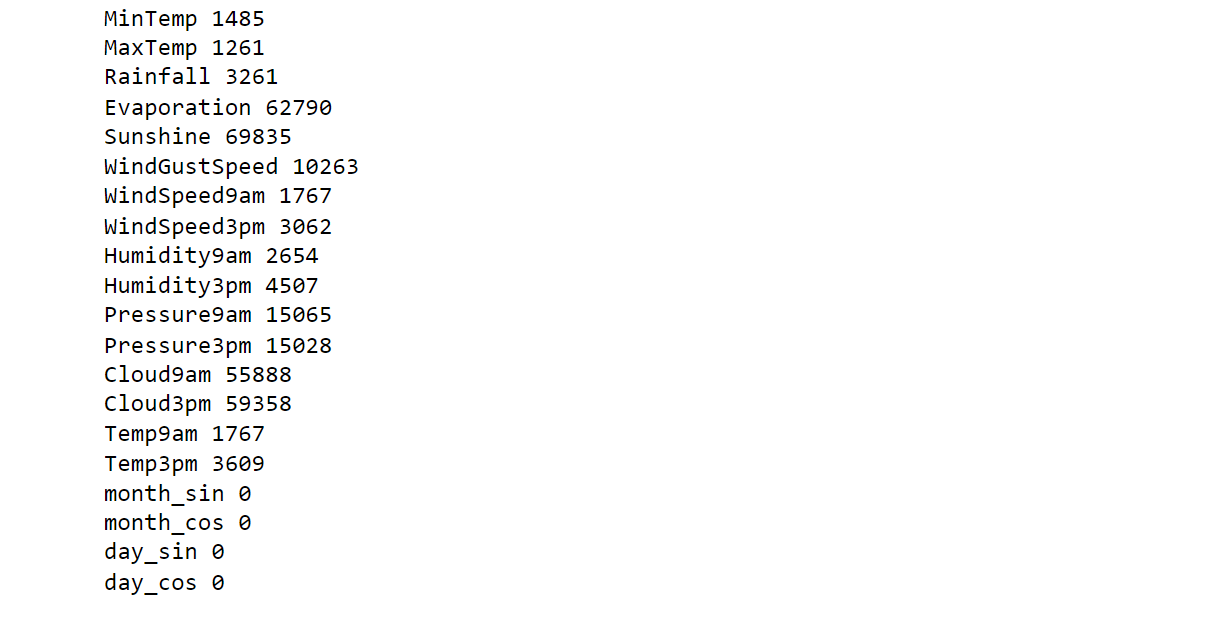
# Numerical variables with missing values


for i in num_col:
    print(i, main_data[i].isnull().sum())
Output:
# Use the column's median value to fill in any missing data
for i in num_col:
main_data[i].fillna(main_data[i].median(), inplace=True)
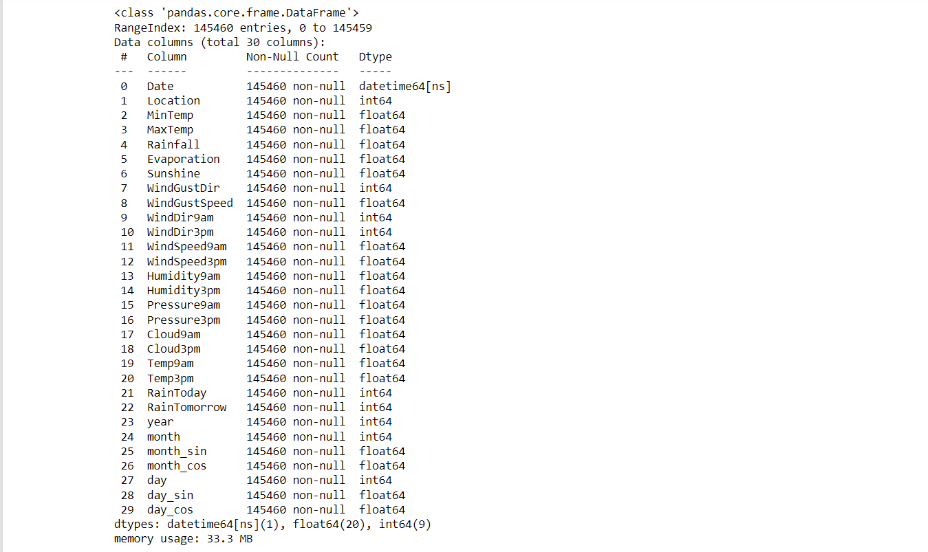
main_data.info()
Output:
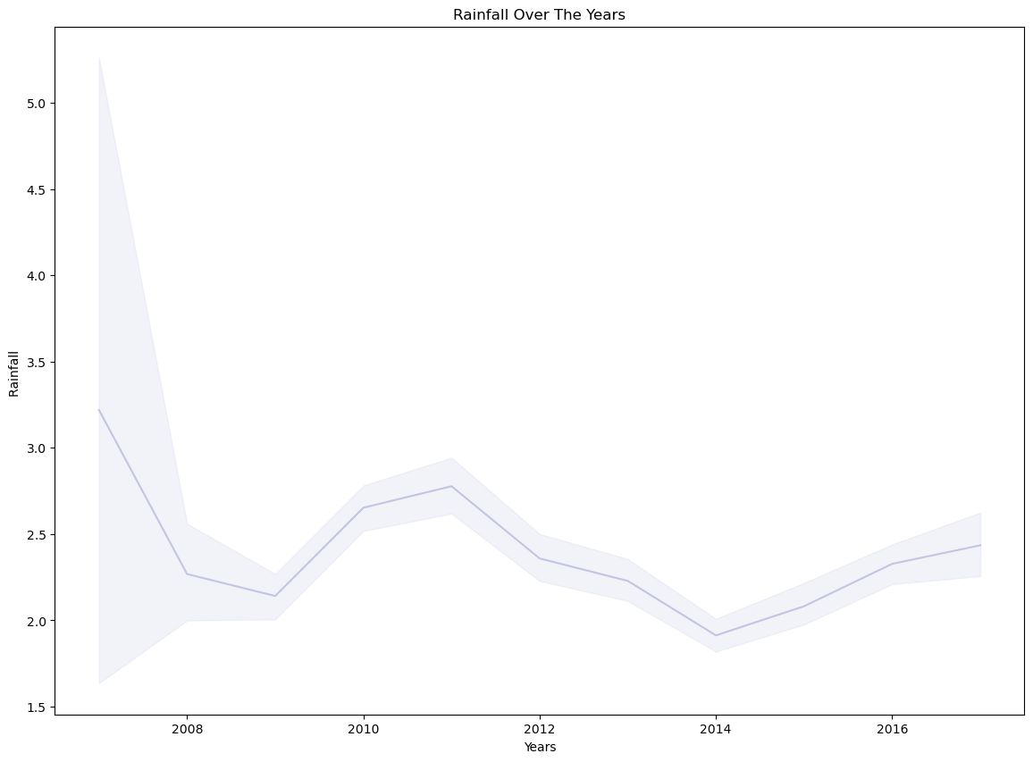
#calculating a line plot of annual rainfall over many years
plt.figure(figsize=(14,10))
Time_s=sns.lineplot(x=main_data['Date'].dt.year,y="Rainfall",data=main_data,color="#C2C4E2")
Time_s.set_title("Rainfall Over The Years")
Time_s.set_ylabel("Rainfall ")
Time_s.set_xlabel("Years")
Output:
Text(0.5, 0, 'Years')
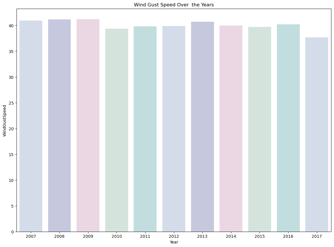
#evaluating the average annual speed of wind gusts over the years
colours = ["#D0DBEE", "#C2C4E2", "#EED4E5", "#D1E6DC", "#BDE2E2"]
plt.figure(figsize=(14,10))
Week_days=sns.barplot(x=main_data['Date'].dt.year,y="WindGustSpeed",data=main_data, ci =None,palette = colours)
Week_days.set_title("Wind Gust Speed Over  the Years")
Week_days.set_ylabel("WindGustSpeed")
Week_days.set_xlabel("Year")
Output:
Text(0.5, 0, 'Year')
Data Preprocessing
Data preprocessing is an important step in machine learning for predicting rainfall. It involves cleaning, transforming, and organizing the data so that it can be effectively used to train a machine-learning model.
Here we will take the following actions:
- Removing missing or invalid data: This can include removing rows or columns with missing values or replacing missing values with a placeholder value.
- Data transformation: This includes converting categorical data into numerical data, as well as creating new features from the existing data.
- Splitting of Data
- Normalisation of Data
- Outcasting outliers
# A table holding category data should have labels in each column.
label_encoder = LabelEncoder()
for i in object_col:
    main_data[i] = label_encoder.fit_transform(main_data[i])

main_data.info()
Output:
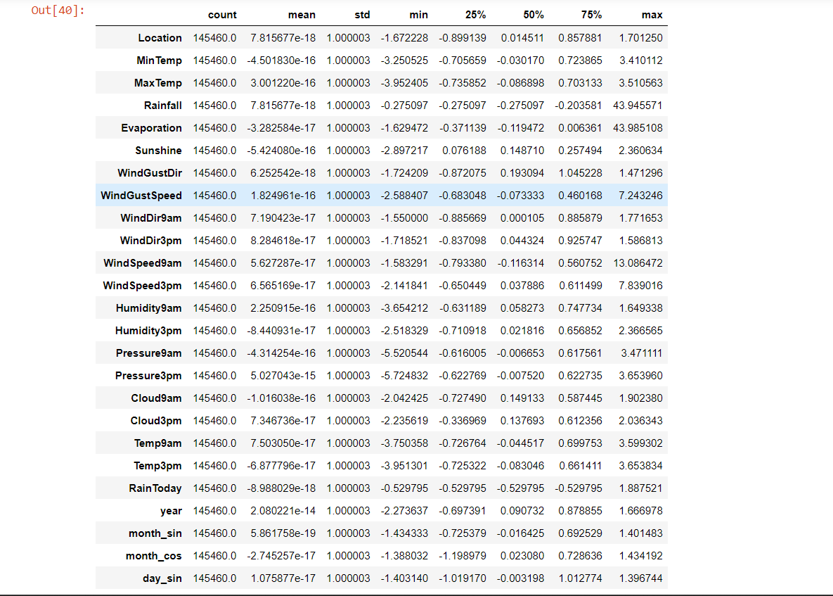
# Preparation for the attributes of Scale Data


features_ = main_data.drop(['RainTomorrow', 'Date', 'day', 'month'], axis=1)


target_ = main_data['RainTomorrow']


#For the features, set up a standard scaler.
col_names = list(features_.columns)
standard_scaler = preprocessing.StandardScaler()
features_ = standard_scaler.fit_transform(features_)
features_ = pd.DataFrame(features_, columns=col_names)


features_.describe().T
Output:
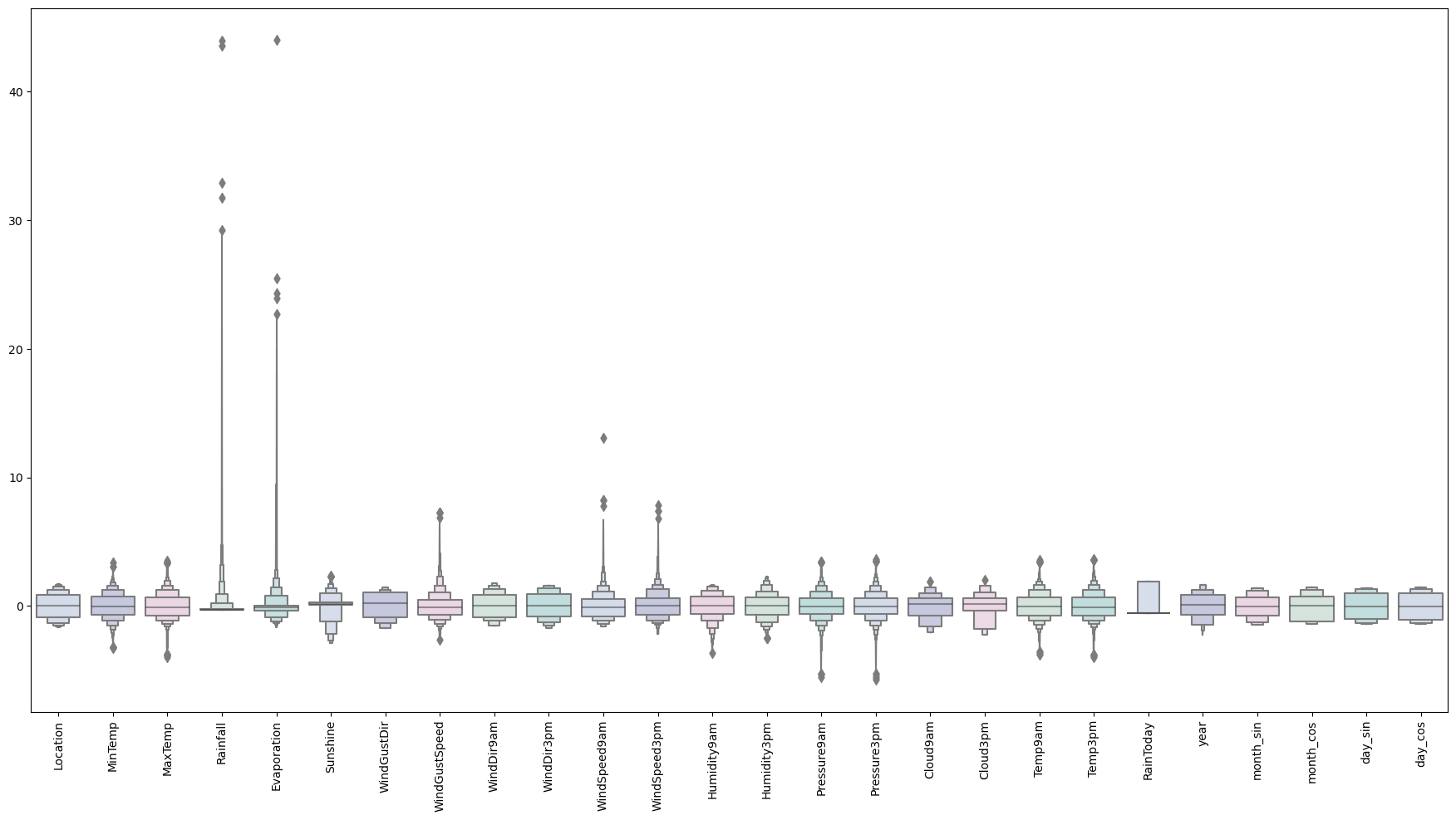
#Finding outliers
#examining the enlarged features
colours = ["#D0DBEE", "#C2C4E2", "#EED4E5", "#D1E6DC", "#BDE2E2"]
plt.figure(figsize=(22,11))
sns.boxenplot(data = features_,palette = colours)
plt.xticks(rotation=90)
plt.show()
Output:
# totatl data
features_["RainTomorrow"] = target_


# Outlier Dropping


features_ = features_[(features_["MinTemp"]<2.3)&(features_["MinTemp"]>-2.3)]
features_ = features_[(features_["MaxTemp"]<2.3)&(features_["MaxTemp"]>-2)]
features_ = features_[(features_["Rainfall"]<4.5)]
features_ = features_[(features_["Evaporation"]<2.8)]
features_ = features_[(features_["Sunshine"]<2.1)]
features_ = features_[(features_["WindGustSpeed"]<4)&(features_["WindGustSpeed"]>-4)]
features_ = features_[(features_["WindSpeed9am"]<4)]
features_ = features_[(features_["WindSpeed3pm"]<2.5)]
features_ = features_[(features_["Humidity9am"]>-3)]
features = features_[(features_["Humidity3pm"]>-2.2)]
features_ = features_[(features_["Pressure9am"]< 2)&(features_["Pressure9am"]>-2.7)]
features_ = features_[(features_["Pressure3pm"]< 2)&(features_["Pressure3pm"]>-2.7)]
features_ = features_[(features_["Cloud9am"]<1.8)]
features_ = features_[(features_["Cloud3pm"]<2)]
features_ = features_[(features_["Temp9am"]<2.3)&(features_["Temp9am"]>-2)]
features_ = features_[(features_["Temp3pm"]<2.3)&(features_["Temp3pm"]>-2)]


features_.shape
Output:

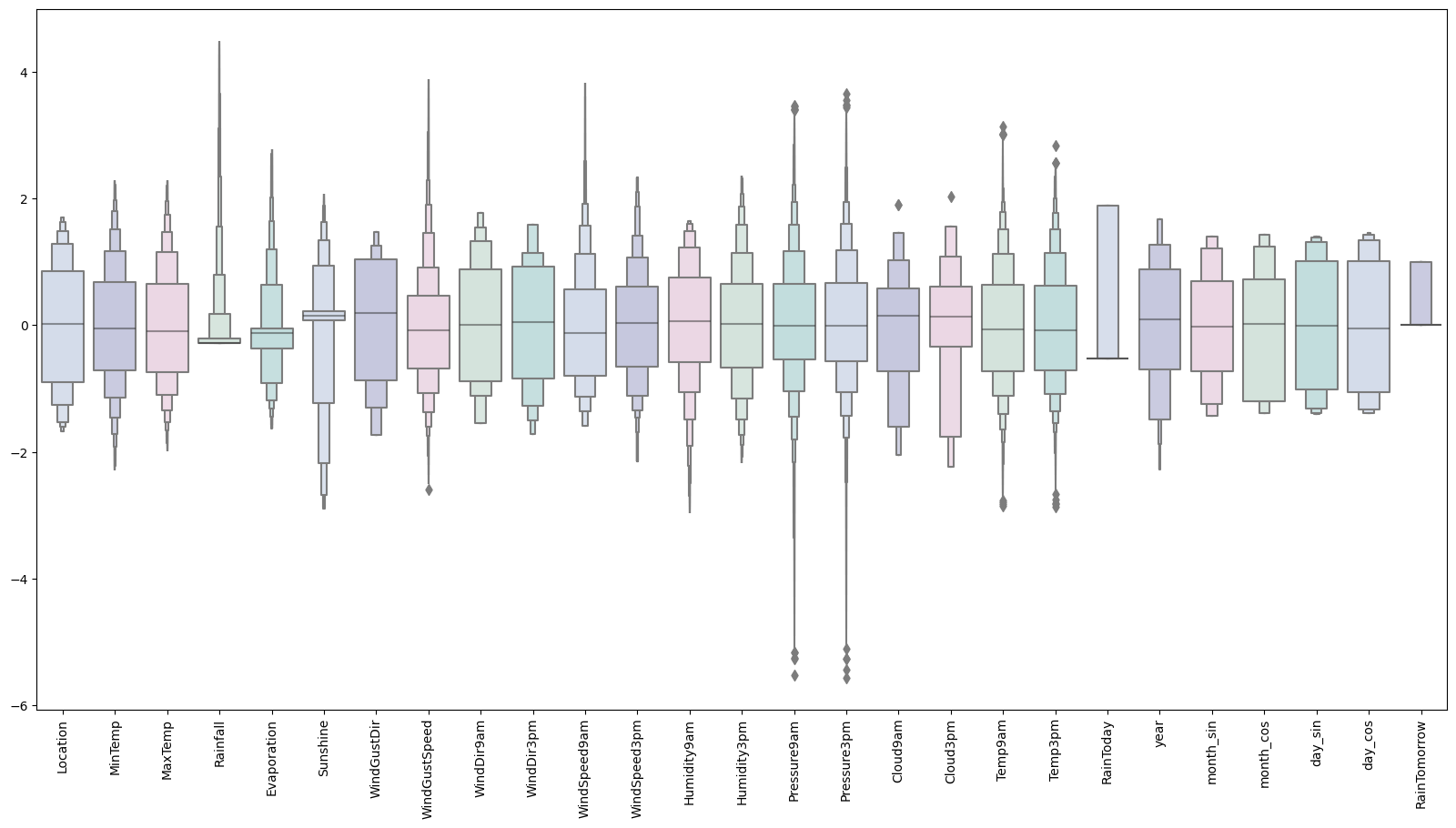
# Observing the scaled features without outliers
colours = ["#D0DBEE", "#C2C4E2", "#EED4E5", "#D1E6DC", "#BDE2E2"]
plt.figure(figsize=(20,10))
sns.boxenplot(data = features,palette = colours)
plt.xticks(rotation=90)
plt.show()
Output:
Modeling
Model building is an important step in machine learning for predicting rainfall using an Artificial Neural Network (ANN). The process of model building typically involves the following steps:
- Defining the ANN's design entails deciding on its number of layers, the number of neurons that will be present in each layer, and the activation functions that will be applied.
- The weights and biases of the network's neurons are modified using a training dataset so that the ANN can forecast rainfall with accuracy.
- Utilizing a validation dataset to gauge the ANN's performance entails determining how accurate its predictions are.
- Adjusting the ANN's hyperparameters and architecture may be done to boost its performance based on the evaluation's findings.
- Testing the ANN: The last stage is to evaluate the ANN's performance using an unused test dataset.
X = features_.drop(["RainTomorrow"], axis=1)
y = features_["RainTomorrow"]


# Splitting test and training sets
X_train, X_test, y_train, y_test = train_test_split(X, y, test_size = 0.2, random_state = 42)


X.shape
Output:

#Early stopping
early_stopping = callbacks.EarlyStopping(
min_delta=0.001,
patience=20,
restore_best_weights=True,
)
# Initialising the NN
model_01 = Sequential()
# layers
model_01.add(Dense(units = 32, kernel_initializer = 'uniform', activation = 'relu', input_dim = 26))
model_01.add(Dense(units = 32, kernel_initializer = 'uniform', activation = 'relu'))
model_01.add(Dense(units = 16, kernel_initializer = 'uniform', activation = 'relu'))
model_01.add(Dropout(0.25))
model_01.add(Dense(units = 8, kernel_initializer = 'uniform', activation = 'relu'))
model_01.add(Dropout(0.5))
model_01.add(Dense(units = 1, kernel_initializer = 'uniform', activation = 'sigmoid'))
# Compiling the ANN
opt = Adam(learning_rate=0.00009)
model_01.compile(optimizer = opt, loss = 'binary_crossentropy', metrics = ['accuracy'])
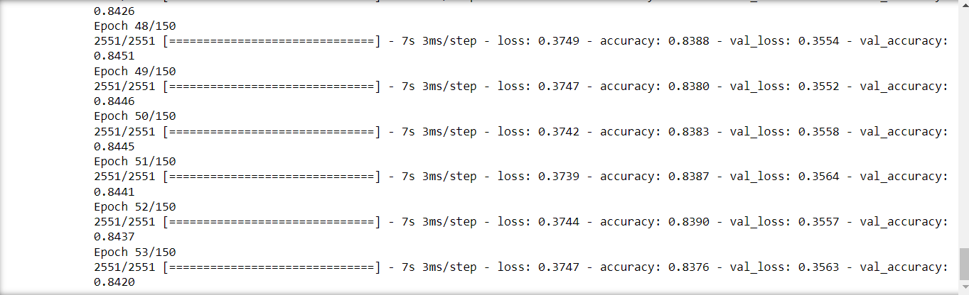
# Train the ANN
history = model_01.fit(X_train, y_train, batch_size = 32, epochs = 150, callbacks=[early_stopping], validation_split=0.2)
Output:
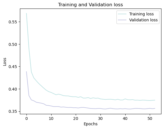
history_af = pd.DataFrame(history.history)


plt.plot(history_af.loc[:, ['loss']], "#BDE2E2", label='Training loss')
plt.plot(history_af.loc[:, ['val_loss']],"#C2C4E2", label='Validation loss')
plt.title('Training and Validation loss')
plt.xlabel('Epochs')
plt.ylabel('Loss')
plt.legend(loc="best")


plt.show()
Output:
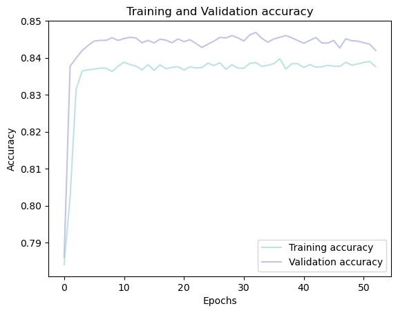
history_af = pd.DataFrame(history.history)


plt.plot(history_af.loc[:, ['accuracy']], "#BDE2E2", label='Training accuracy')
plt.plot(history_af.loc[:, ['val_accuracy']], "#C2C4E2", label='Validation accuracy')


plt.title('Training and Validation accuracy')
plt.xlabel('Epochs')
plt.ylabel('Accuracy')
plt.legend()
plt.show()
Output:
# Predicting the test set
y_pred = model_01.predict(X_test)
y_pred = (y_pred > 0.5)
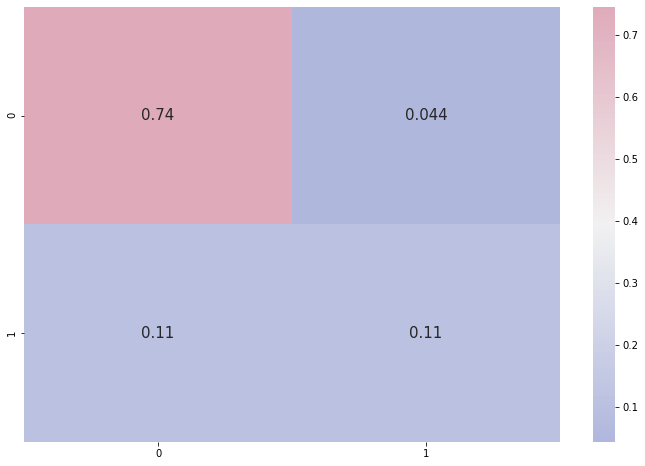
# confusion matrix
cmap_1 = sns.diverging_palette(260,-10,s=50, l=75, n=5, as_cmap=True)
plt.subplots(figsize=(12,8))
cf_matrix_01 = confusion_matrix(y_test, y_pred)
sns.heatmap(cf_matrix_01/np.sum(cf_matrix_01), cmap = cmap_1, annot = True, annot_kws = {'size':15})
Output:
<AxesSubplot:>
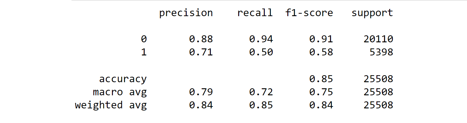
print(classification_report(y_test, y_pred))
Output:
Despite these challenges, machine learning has shown great potential for improving the accuracy of rainfall predictions. By using advanced machine learning techniques, such as ANNs, SVMs, and decision trees, researchers have been able to achieve high levels of accuracy in their predictions. However, there is still much work to be done in order to fully realize the potential of machine learning for rainfall prediction.
In conclusion, Rainfall prediction using machine learning is a complex task that requires the handling of large datasets, preprocessing and advanced machine learning models. Researchers are constantly working to improve the accuracy and reliability of these predictions. Techniques such as ANNs, SVMs, decision trees, Random Forests, and Gradient Boosting are being used with good results, but there is still much room for improvement. With more data and continued advancements in machine learning algorithms, we can expect to see even more accurate and reliable rainfall predictions in the future.