Random Forest Algorithm for Machine Learning

Introduction to Random Forest

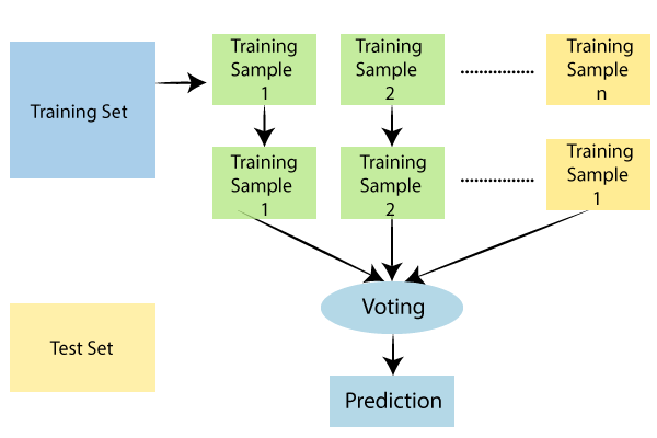
Random forest is an ensemble-based supervised learning model. The concept of random forest is used in both classifications as well as in the regression problems. Basically, in ensemble-based learning, multiple algorithms are combined to build a robust prediction model, such that these algorithms can be similar or even dissimilar ones.

Similarly, random forest joins multiple decision trees constructing a forest which will act as an ensemble. Each of these individual trees helps to output a prediction of class, and the one with maximum votes wins becoming the model's prediction.    

Working of Random Forest:

1. We will first start by selecting a random sample from the dataset.
2. Then we will create decision trees individually for every single record/ sample, so as to get the output from each of the decision trees.
3. Next, we will perform voting for each of the predicted results.
4. And at the end, the most voted predicted the result would be selected as a final result.

Advantages of Random Forest:

1. Since each of the decision trees is trained on a given dataset, so the prediction depends on the power of the crowd, which makes it an unbiased model.
2. It is one of the most stable algorithms means it does not get affected with an addition of any new data point to the dataset. It may hinder one of the decision trees, but it will not have an impact on the rest of the decision trees in the forest.
3. It performs well with both categorical and numerical data.
4. It also works well with the scaled values.

Disadvantages of Random Forest:

1. As there is a group of decision trees in the Random forest, the requirement of resources also increases, which further increases the complexity of the algorithm.
2. It takes a lot of time to train the model as compared to other algorithms.

Implementation of Random Forests:

We will now see how random forest works. So, we will start by importing the libraries and dataset. And then, we will pre-process the dataset as we did in earlier models.

# Importing the libraries
 import numpy as np
 import matplotlib.pyplot as plt
 import pandas as pd
 
# Importing the dataset
 dataset = pd.read_csv('Social_Network_Ads.csv')
 X = dataset.iloc[:, [2, 3]].values
 y = dataset.iloc[:, 4].values 
 
#Data Pre-Processing
 # Splitting the dataset into the Training set and Test set
 from sklearn.model_selection import train_test_split
 X_train, X_test, y_train, y_test = train_test_split(X, y, test_size = 0.25, random_state = 0)
 
# Feature Scaling
 from sklearn.preprocessing import StandardScaler 
 sc = StandardScaler()
 X_train = sc.fit_transform(X_train)
 X_test = sc.transform(X_test) 

Now that we are done with data pre-processing, we will start fitting random forest classification to the training set, and for that, we will create a classifier. We will first import the RandomForestClassifier class from the sklearn.ensemble library. Then we will create a variable “classifier” which is an object of RandomForestClassifier. To this we will pass the following parameters;

1. The very first parameter is the n_estimators that is the no of trees in a forest that is going to predict if the user will buy or not the SUV, is set to 10 trees by default.
2. The second parameter is the criterion equals to entropy, which we also used in the decision tree model as it evaluates the quality of the split. The more the homogenous is the group of users, the more entropy would be reduced.
3. And the last one is the random_state, which is set to 0, to get the same results.

And then, we will fit the classifier to the training set using the fit method so as to make the classifier learn the correlations between X_train and y_train. 

# Fitting Random Forest Classification to the Training set
from sklearn.ensemble import RandomForestClassifier
classifier = RandomForestClassifier(n_estimators = 10, criterion = 'entropy', random_state = 0)
classifier.fit(X_train, y_train) 

We will now predict the observations after the classifier learns the correlation. We will create a variable named y_pred, which is the vector of prediction that contains the predictions of test_set results, followed by creating confusion metrics as we did in the previous models.

# Predicting the Test set results
y_pred = classifier.predict(X_test)
# Making the Confusion Matrix
from sklearn.metrics import confusion_matrix
cm = confusion_matrix(y_test, y_pred) 

Output:

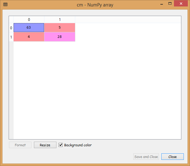
From the image given above, we can see that we have only nine incorrect predictions, which is quite good.

In the end, we will visualize the training set, and test set results, as we have done in the previous models. We will plot a graph that will differentiate the region, which predicts for the users who will buy the SUV from the region, which predicts the users who will not buy an SUV.  

Visualizing the Training Set results:

Here we are going to visualize the training set results. In this we will have a graphical visualization that will predict Yes for the users who will buy the SUV and No for the users who will not purchase the SUV, in the similar way as done before. 

# Visualising the Training set results
 from matplotlib.colors import ListedColormap
 X_set, y_set = X_train, y_train
 X1, X2 = np.meshgrid(np.arange(start = X_set[:, 0].min() - 1, stop = X_set[:, 0].max() + 1, step = 0.01),
                      np.arange(start = X_set[:, 1].min() - 1, stop = X_set[:, 1].max() + 1, step = 0.01))
 plt.contourf(X1, X2, classifier.predict(np.array([X1.ravel(), X2.ravel()]).T).reshape(X1.shape),
              alpha = 0.75, cmap = ListedColormap(('red', 'green'))) 
 plt.xlim(X1.min(), X1.max())
 plt.ylim(X2.min(), X2.max())
 for i, j in enumerate(np.unique(y_set)):
     plt.scatter(X_set[y_set == j, 0], X_set[y_set == j, 1],
                 c = ListedColormap(('red', 'green'))(i), label = j)
 plt.title('Random Forest Classification (Training set)')
 plt.xlabel('Age')
 plt.ylabel('Estimated Salary')
 plt.legend()
 plt.show() 

Output:

From the output image given above, the points here are true results such that each point corresponds to each user of the Socical_Network (users in the dataset), and the region here are the predictions i.e., the red region contains all the users for which the classifier will predict the user does not purchase the SUV and green region contains all the user where the classifier predicts the user will buy an SUV.

The prediction boundary is the region limit between the red and green regions. We can clearly see we have a different prediction boundary then the previous classifiers. 

For each user, we have ten trees in our forest that predicted Yes if the user bought the SUV or NO if the user didn't buy the SUV. In the previous decision tree model, we have only one tree that was making the prediction, but in the existing model, we have ten trees. After the ten trees make the predictions, they then undergo the majority voting. And so, the random forest makes the predictions Yes or No based on the majority of votes.

We can see most of the red, as well as green users, are well classified in the red region and green region, respectively. Since it is a training set, we have very few incorrect predictions.  In the next step, we will see if this Over fitting issue compromises the test set result or not.

Visualizing the Test Set results:

Now we will visualize the same for the test set.

# Visualising the Test set results
 from matplotlib.colors import ListedColormap
 X_set, y_set = X_test, y_test
 X1, X2 = np.meshgrid(np.arange(start = X_set[:, 0].min() - 1, stop = X_set[:, 0].max() + 1, step = 0.01),
                      np.arange(start = X_set[:, 1].min() - 1, stop = X_set[:, 1].max() + 1, step = 0.01))
 plt.contourf(X1, X2, classifier.predict(np.array([X1.ravel(), X2.ravel()]).T).reshape(X1.shape),
              alpha = 0.75, cmap = ListedColormap(('red', 'green')))
 plt.xlim(X1.min(), X1.max())
 plt.ylim(X2.min(), X2.max())
 for i, j in enumerate(np.unique(y_set)):
     plt.scatter(X_set[y_set == j, 0], X_set[y_set == j, 1],
                 c = ListedColormap(('red', 'green'))(i), label = j)
 plt.title('Random Forest Classification (Test set)')
 plt.xlabel('Age')
 plt.ylabel('Estimated Salary') 
 plt.legend()
 plt.show() 

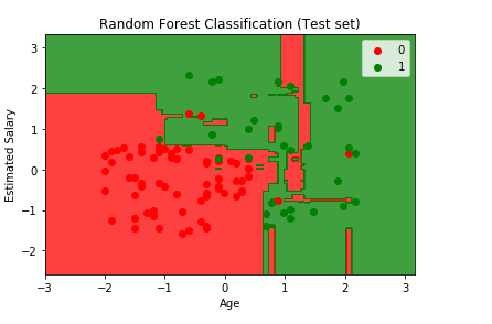
From the above output image, we can see that it is a case of Overfitting, as the red region was made to catch the red users who didn’t buy the SUV, and the green region was meant for the green users who purchased the SUV. But unfortunately, the red region is containing some of the users who bought the SUV, and the green region includes the user who didn’t purchase the SUV.

The model learned how to classify the training set, but it couldn’t make it for new observations. So, from this, it can be concluded among all the classifiers that we studied so far, the Kernel SVM classifier, and the Naïve Bayes classifier gives the most promising result, as they have a smooth curved prediction boundary that was catching correct users in the right region. Also, there was no such issue of Overfitting as it occurred in the current model while predicting new users in the test set.

Conclusion:

There is always a battle while choosing a correct model based on the highest accuracy (having the maximum no of correct predictions) and preventing Overfitting. It is very much clear that we want to prevent Overfitting, and also in a situation like this, Kernel SVM is the best among all the classifiers because it has good accuracy with very few incorrect predictions.

It actually caught the red users in the red region and green users in the green region without having the Overfitting issue for the new observations. The Kernel SVM classifier is better than the logistic regression classifier and the SVM classifier because it encompassed the red users in the red region without including the green users in the red region, or vice versa.