Support Vector Machines

Introduction to SVM

Support Vector Machines are part of the supervised learning model with an associated learning algorithm. It is the most powerful and flexible algorithm used for classification, regression, and detection of outliers. It is used in case of high dimension spaces, where each data item is plotted as a point in n-dimension space such that each feature value corresponds to the value of specific coordinate.

The classification is made on the basis of a hyperplane/line as wide as possible, which distinguishes between two categories more clearly. Basically, support vectors are the observational points of each individual, whereas the support vector machine is the boundary that differentiates one class from another class. 

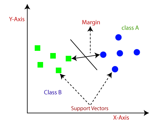
Some significant terminology of SVM are given below:-

• Support Vectors: These are the data point or the feature vectors lying nearby to the hyperplane. These help in defining the separating line. 
• Hyperplane: It is a subspace whose dimension is one less than that of a decision plane. It is used to separate different objects into their distinct categories. The best hyperplane is the one with the maximum separation distance between the two classes.   
• Margins: It is defined as the distance (perpendicular) from the data point to the decision boundary. There are two types of margins: good margins and margins. Good margins are the one with huge margins and the bad margins in which the margin is minor.

The main goal of SVM is to find the maximum marginal hyperplane, so as to segregate the dataset into distinct classes. It undergoes the following steps:

• Firstly the SVM will produce the hyperplanes repeatedly, which will separate out the class in the best suitable way. 
• Then we will look for the best option that will help in correct segregation.

Advantages of SVM

• Effective in handling large no of feature vectors.
• Nonlinear data can be handled, incorporating the concept of kernels in SVM, as kernels are the strength of SVM. 
• Robust model as it maximizes the margins.
• Low-risk factor of Overfitting.
• SVM results better in comparison to ANN.

Disadvantages of SVM

• Appropriate kernel to be selected, as an incorrect kernel may lead to errors in the results.
• Larger the sample, poor the performance.
• Extremely slow in the test phase.
• Due to the implementation of quadratic programming, the complexity of SVM increases, and it requires more memory.

Applications of SVM

• Facial expression classification, as it incorporates statistical models of shapes and SVM’s.
• Speech Recognition as the SVM accepts the keywords and rejects the non-keywords.
• Handwritten character recognition.
• Hypertext and text categorization.

Concept of Kernels in SVM

With the help of the Kernel trick, SVM can translate the input data space into the desired output space. It is fundamentally used to change a low dimensional space into a higher dimension space, or we can say it transforms a non-separable problem into a separable problem simply by changing its dimensions. It is more powerful and flexible, such that it provides more accurate results.

Types of the kernel:

There are three types of kernels given below:

1. Linear Kernel
2. Polynomial Kernel
3. Radial Basis Function Kernel

Linear Kernel: It is a dot product of the two observations (X, Y) with an addition of a constant optionally. It is one of the simplest methods of the kernel. Mathematically it can be written as;

K(X, Y) = X^TY + C

Polynomial Kernel: It is a non-stationary kernel.  It is best suited when the training data is in normalized form. It can be mathematically written as;

K(X, Y) = (?X^TY+C) ^D

Where ? is the adjustable parameter, it is termed as slope, C is the constant, and D is the degree of the polynomial.

Radial Basis Function Kernel: It is also called a Gaussian Kernel. It is the most commonly used SVM kernel. It maps the input space to an indefinite dimension space. Mathematically it is given as; 

K(X, Y) = exp (-gamma*sum(X-Y^2))

We will now see how an SVM classifier segregates two different classes into two different categories, and we will also compare its result with that of the Logistic Regression model. For this, we will take the same dataset Social_Network_Ads that we used in the Logistic regression model in the previous chapter.

It will undergo the same steps till pre-processing as we did earlier:

# Importing the libraries
 import numpy as np
 import matplotlib.pyplot as plt
 import pandas as pd

 # Importing the dataset
 dataset = pd.read_csv('Social_Network_Ads.csv')
 X = dataset.iloc[:, [2, 3]].values
 y = dataset.iloc[:, 4].values

 # Split the dataset into the Training set and Test set 
 from sklearn.model_selection import train_test_split
 X_train, X_test, y_train, y_test = train_test_split(X, y, test_size = 0.25, random_state = 0)

 # Feature Scaling
 from sklearn.preprocessing import StandardScaler
 sc = StandardScaler()
 X_train = sc.fit_transform(X_train)
 X_test = sc.transform(X_test) 

After we are done with feature scaling, we will now fit the classifier to the training set. For this, we will first need to create an SVM classifier. And so we will import the SVC library from scikit learn. We will create a variable named classifier, which is an object of SVC. We will use 'rbf' kernel, which is also known as the Gaussian Kernel.

It is a highly sophisticated kernel. It will help us in elevating our data into a new Dimension. So, that our data can be linearly separable by a hyperplane in a new dimension, and then we will project our data to 2Dimension to get SVM separator. Since the Kernel SVM algorithm is based on random factors, so here random_state variable is taken as 0 to get the same results. In this way kernel classifier is built. And then, we will fit the classifier to X_train and y_train so that the classifier can learn the correlation between X-train and y_train.

# Fitting classifier to the Training set
sklearn.svm import SVC
classifier=SVC(kernel='rbf',random_state=0)
classifier.fit(X_train,y_train) 

After the classifier learns the correlation, we will now predict the observations. So, for that, we will create a variable y_pred, which is the vector of prediction containing the predictions of test_set results.

y_pred = classifier.predict(X_test)

Now we will create a confusion matrix for which we will import confusion_matrix function from the library of sklearn.metrics. It will contain correct as well as the incorrect predictions. Here our concern is calculating the number of incorrect predictions.

from sklearn.metrics import confusion_matrix
cm = confusion_matrix(y_test, y_pred) 

Output:

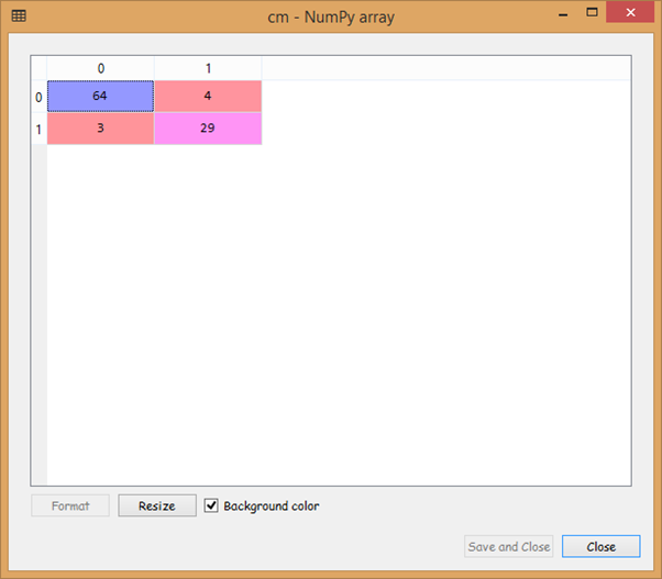
From the output image given above, we can see that we have seven incorrect predictions on the test_set, which is much better than the Logistic Regression model as it was calculating 11 incorrect predictions. So, this proves to be an improved model.

Next, we will visualize the training set results as well as the test set results in the same way as we have done in the previous Logistic Regression model. We are going to plot a graph that will differentiate one region where our model predicts the users will purchase the SUV from the prediction region where the user will not purchase an SUV.

Visualising the Training set results:

Now we will have a graphical visualization of the training set results. For this we will plot a graph where our SVM model will predict Yes for the users who will purchase the SUV and No for the users who will not buy the SUV, and will be carried out in a same way as we did in the previous model.

# Visualising the Training set results
 from matplotlib.colors import ListedColormap
 X_set, y_set = X_train, y_train
 X1, X2 = np.meshgrid(np.arange(start = X_set[:, 0].min() - 1, stop = X_set[:, 0].max() + 1, step = 0.01),
                      np.arange(start = X_set[:, 1].min() - 1, stop = X_set[:, 1].max() + 1, step = 0.01))
 plt.contourf(X1, X2, classifier.predict(np.array([X1.ravel(), X2.ravel()]).T).reshape(X1.shape), 
              alpha = 0.75, cmap = ListedColormap(('red', 'green')))
 plt.xlim(X1.min(), X1.max())
 plt.ylim(X2.min(), X2.max())
 for i, j in enumerate(np.unique(y_set)):
     plt.scatter(X_set[y_set == j, 0], X_set[y_set == j, 1], 
                 c = ListedColormap(('red', 'green'))(i), label = j)
 plt.title('Classifier (Training set)')
 plt.xlabel('Age')
 plt.ylabel('Estimated Salary')
 plt.legend()
 plt.show() 

Output:

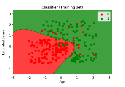
From the output image given above, it can be seen that all the points here are the observation points in a training set, or we can simply say the users of a training set. The red points are the users who didn’t buy the SUV, whereas the green points are the users who bought the SUV. Also, we have prediction regions here, such that the red region indicates the region for the user who will not buy the SUV, and the green region specifies the users who will purchase the SUV.

The separator that is separating the prediction region is called as prediction boundary. Since we built a non-linear classifier, the boundary is not a straight line but is a curve. Both the older users with low estimated salaries and young users with high estimated salaries are classified into the right regions, respectively, by the classifier. There are some incorrect predictions too because our classifier is not an Overfitting classifier, but it is a sensible classifier. The curve has actually separated the data very well.

Visualizing the Test set results:

Now we will visualize the test set results, exactly the same way as done in logistic regression model.

# Visualising the Test set results
 from matplotlib.colors import ListedColormap
 X_set, y_set = X_test, y_test
 X1, X2 = np.meshgrid(np.arange(start = X_set[:, 0].min() - 1, stop = X_set[:, 0].max() + 1, step = 0.01),
                      np.arange(start = X_set[:, 1].min() - 1, stop = X_set[:, 1].max() + 1, step = 0.01))
 plt.contourf(X1, X2, classifier.predict(np.array([X1.ravel(), X2.ravel()]).T).reshape(X1.shape),
              alpha = 0.75, cmap = ListedColormap(('red', 'green'))) 
 plt.xlim(X1.min(), X1.max())
 plt.ylim(X2.min(), X2.max())
 for i, j in enumerate(np.unique(y_set)):
     plt.scatter(X_set[y_set == j, 0], X_set[y_set == j, 1],
                 c = ListedColormap(('red', 'green'))(i), label = j)
 plt.title('Classifier (Test set)')
 plt.xlabel('Age')
 plt.ylabel('Estimated Salary') 
 plt.legend()
 plt.show() 

Output:

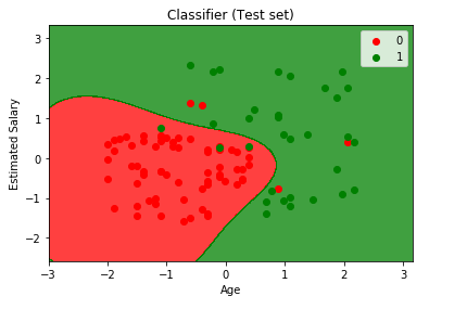
From the output given above, we can see that almost all our new observations are classified into right category. The Kernel SVM made a great deal of prediction predicting the users who wouldn’t buy the SUV in red region and the user who would buy the SUV in green region. As we counted 7 incorrect predictions in the confusion matrix, same we can see from the output image and count them. Since it classified very well, so we can confirm it is a good classifier.