Text Classification- Machine Learning
Text classification is a common task in natural language processing and machine learning, which involves assigning predefined categories or labels to a given text. This can be done using various techniques such as supervised learning, unsupervised learning, and deep learning. Common algorithms used for text classification include:
- Naive Bayes
- Support Vector Machines (SVMs)
- Random Forests
- Neural networks (such as convolutional neural networks or recurrent neural networks)

The process of text classification typically includes pre-processing the text data, such as tokenization and feature extraction, training a model using labeled data, and evaluating the performance of the model using metrics such as accuracy, precision, recall, and f1-score.
Here, we will classify text with Keras and now we will perform it through code.
Importing Libraries
from sklearn.feature_extraction.text import CountVectorizer
from sklearn.preprocessing import LabelEncoder
from sklearn.preprocessing import OneHotEncoder
from sklearn.model_selection import RandomizedSearchCV
from sklearn.model_selection import train_test_split
from sklearn.linear_model import LogisticRegression


import pandas as pd
import tensorflow as tf
import matplotlib.pyplot as plt
import numpy as np


from tensorflow.keras.wrappers.scikit_learn import KerasClassifier
from tensorflow.keras.preprocessing.text import Tokenizer
from tensorflow.keras.models import Sequential
from tensorflow.keras import layers
from tensorflow.keras.preprocessing.sequence import pad_sequences


import os
plt.style.use('ggplot')
Load the data with Pandas after extracting the folder into a data folder:
filepath_dictionary = {'yelp':   'yelp_labelled.txt',
                 'amazon': 'amazon_cells_labelled.txt',
                 'imdb':   'imdb_labelled.txt'}


af_list = []
for source, filepath in filepath_dictionary.items():
    af = pd.read_csv(filepath, names=['sentence', 'label'], sep='\t')
    af['source'] = source
    af_list.append(af)
Exploring the Dataset
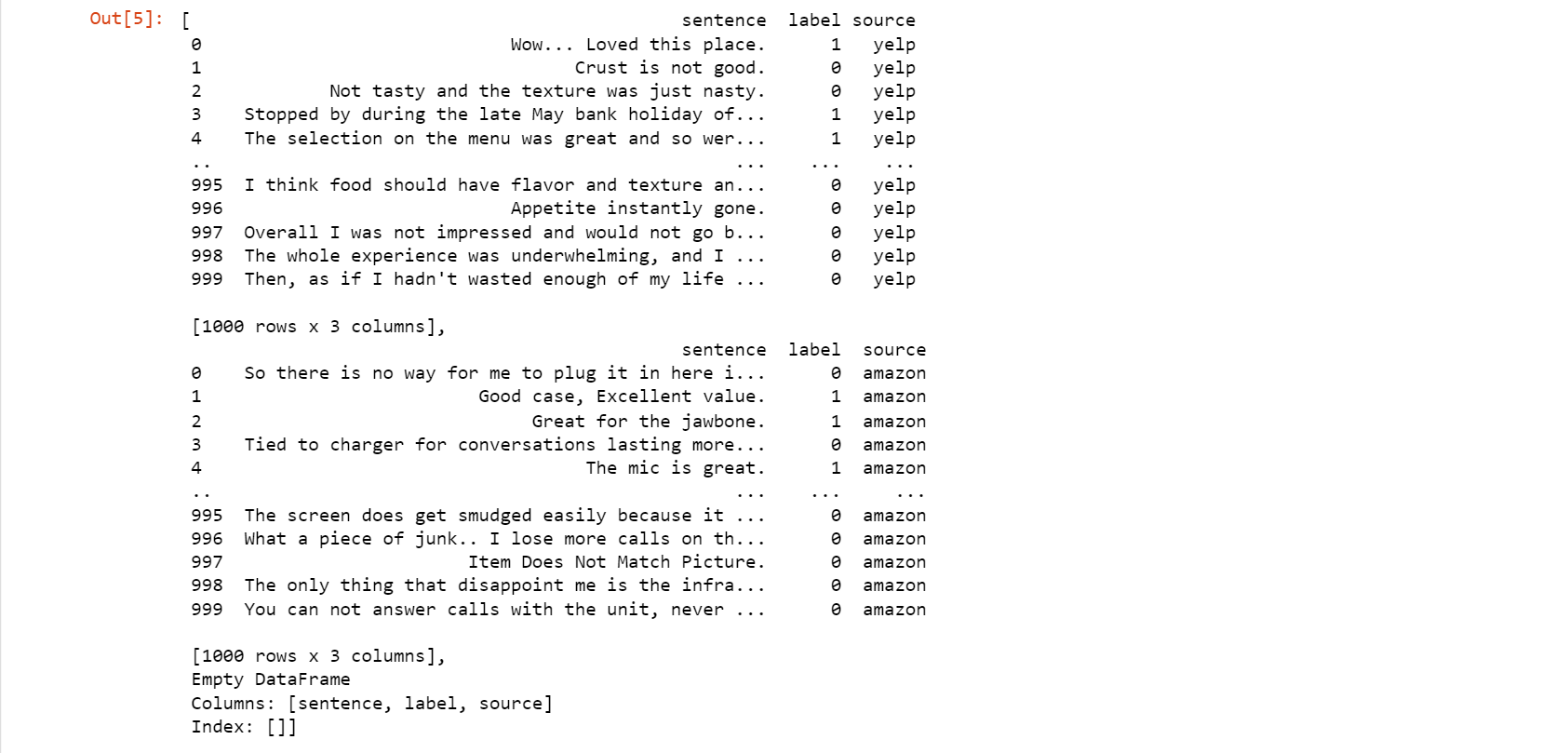
af_list
Output:
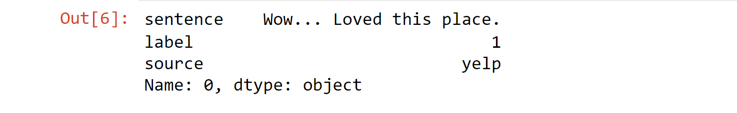
af = pd.concat(af_list)
af.iloc[0]
Output:
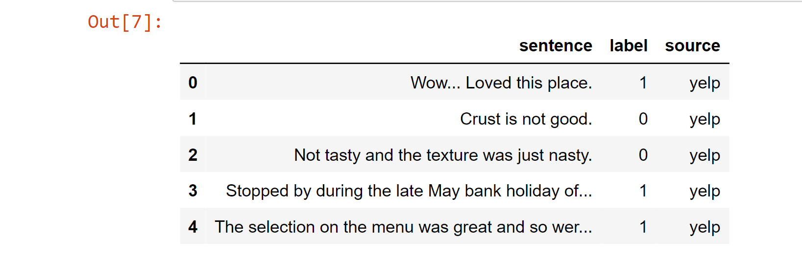
af.head()
Output:
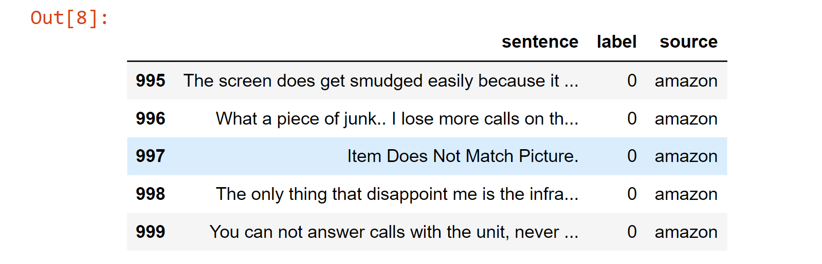
af.tail()
Output:
Now, vectorize phrases using the 'CountVectorizer' function offered by the 'scikit-learn' package. The words in each phrase are used to create a lexicon of all the unique terms used in the sentences. The feature vector of the word count may then be created using this vocabulary:
sent = ['Rashmi likes ice cream', 'Rashmi hates chocolate.']


vect = CountVectorizer(min_df=0, lowercase=False)
vect.fit(sent)
vect.vocabulary_
Output:

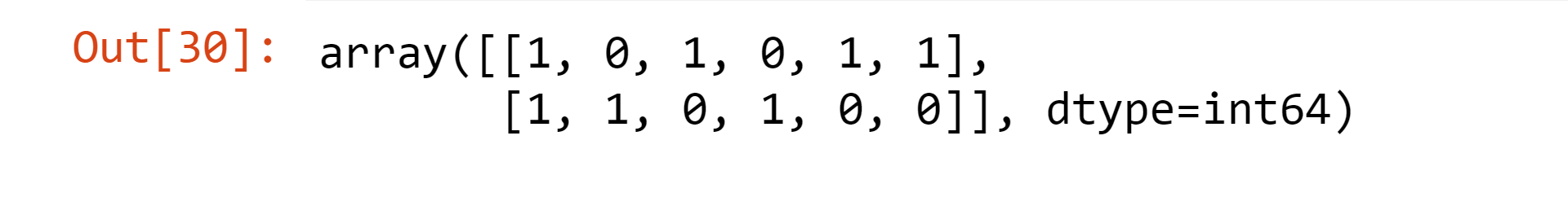
vect.transform(sent).toarray()
Output:
Defining a Baseline Model
First, we'll divide the data into a training and testing set so you can assess the precision and determine whether your model generalizes effectively. This refers to whether the model can successfully operate on data that it has never encountered before. This can help determine whether the model is overfitted.
A model is considered to overfit when it has been overtrained on the training data. Overfitting should be avoided since it would suggest that the model has mostly remembered the training set of data. Due to this, the training data accuracy was high, but the testing data accuracy was poor.
Starting with the Yelp data set that we have combined with our concatenated data collection. The phrases and labels are then taken from there.
af_yelp = af[af['source'] == 'yelp']
sent = af_yelp['sentence'].values
y = af_yelp['label'].values.astype('int')


sent_train, sent_test, y_train, y_test = train_test_split(sent, y, test_size=0.25, random_state=1000)
In order to create the feature vectors for the training and testing set's sentences, do the following:
vect = CountVectorizer()
vect.fit(sent_train)


X_train = vect.transform(sent_train)
X_test  = vect.transform(sent_test)


X_train
Output:

Tokenization is done by CountVectorizer, breaking down the phrases into a collection of tokens. It also gets rid of punctuation and other special characters, and it may also give each word additional preprocessing. To enhance the efficiency of our model, we may choose to utilize a certain tokenizer from the NLTK library using the CountVectorizer or one of the many modifications available to us.
We are going to use a classification model called logistic regression, which is a simple but effective linear model that, technically, is truly a form of regression between 0 and 1 based on the input feature vector. The cutoff value, which is by default set at 0.5, is utilized by the regression model to do classification.
classifier_LR = LogisticRegression()
classifier_LR.fit(X_train, y_train)
score = classifier_LR.score(X_test, y_test)


print("Accuracy:", score)
Output:

You can see that the logistic regression achieved an outstanding 79.6%; nevertheless, let's examine how this model works with the additional datasets that we have. For each of the datasets we have, we run through the entire procedure in this script and analyze it.
for source in af['source'].unique():
    af_source = af[af['source'] == source]
    sent = af_source['sentence'].values
    y = af_source['label'].values.astype('int')


    sent_train, sent_test, y_train, y_test = train_test_split(
        sent, y, test_size=0.25, random_state=1000)


    vect = CountVectorizer()
    vect.fit(sent_train)
    X_train = vect.transform(sent_train)
    X_test  = vect.transform(sent_test)


    classifier_LR = LogisticRegression()
    classifier_LR.fit(X_train, y_train)
    score = classifier_LR.score(X_test, y_test)
    print('Accuracy for {} data: {:.4f}'.format(source, score))
Output:

Great! As you can see, the accuracy of this rather straightforward model is respectable.
Deep Neural Networks

Artificial neural networks (ANN) or feedforward neural networks, which are often referred to as neural networks, are computer networks that were roughly modeled after the neural networks in the human brain. They are made up of neurons, also known as nodes, which are linked together.
As a first step, we have a layer of input neurons into which we feed our feature vectors. The results from this layer are then sent forward to a hidden layer. At each connection, we pass the value ahead while multiplying it by weight and adding a bias to the value. Eventually, an output layer with one or more output nodes is reached after each connection has gone through this process.
One node can be used to create a binary classification, but if there are numerous categories, there should be one node for each category:
Keras
François Chollet's Keras is an API for deep learning and neural networks that may be used with Tensorflow (Google), Theano, or CNTK (Microsoft). To paraphrase the fantastic book Deep Learning with Python by François Chollet: “A model-level library called Keras offers advanced building pieces for creating deep-learning models. Low-level operations like tensor manipulation and differentiation are not supported. Instead, it uses the Keras backend engine, which is a specialised, highly efficient tensor library, to do this. (Source)”
It is an excellent method to begin playing around with neural networks without having to build each layer and component individually. Tensorflow, for instance, is a fantastic machine-learning toolkit, but it requires a lot of boilerplate code to execute a model.
First Keras Model
There are two primary models that Keras supports. Both the functional API, which can be used for complex models with extensive network architecture, and the sequential model API, which can carry out all of the Sequential model's operations, are available.
The Sequential model is a stack of linear layers where you may utilize any of the many Keras-compatible layers. The Dense layer—a standard densely coupled neural network layer with all the weights and biases you are already familiar with—is the most common layer.
We must be aware of the input dimension of our feature vectors before we can create our model. Since the subsequent layers are capable of doing automated shape inference, this only occurs in the top layer. The Sequential model may be constructed by sequentially adding layers.
input_dim_ = X_train.shape[1] # Frequency of features
model_0 = Sequential()
model_0.add(layers.Dense(10, input_dim=input_dim_, activation='relu'))
model_0.add(layers.Dense(1, activation='sigmoid'))
model_0.compile(loss='binary_crossentropy',
optimizer='adam',
metrics=['accuracy'])
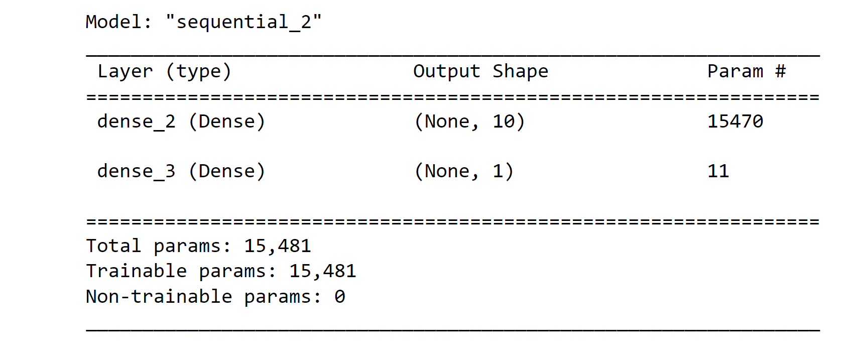
model_0.summary()
Output:
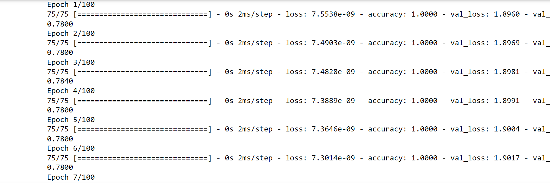
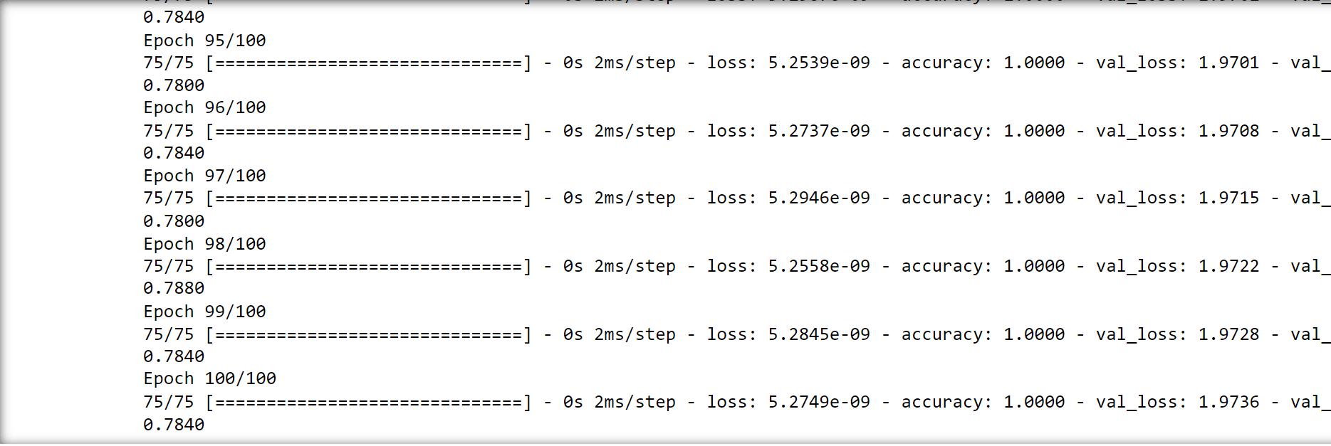
history = model_0.fit(X_train, y_train,
                    epochs=100,
                    verbose=True,
                    validation_data=(X_test, y_test),
                    batch_size=10)
Output:
loss, accuracy = model_0.evaluate(X_train, y_train, verbose=False)
print("Training Accuracy: {:.4f}".format(accuracy))
loss, accuracy = model_0.evaluate(X_test, y_test, verbose=False)
print("Testing Accuracy:  {:.4f}".format(accuracy))
Output:
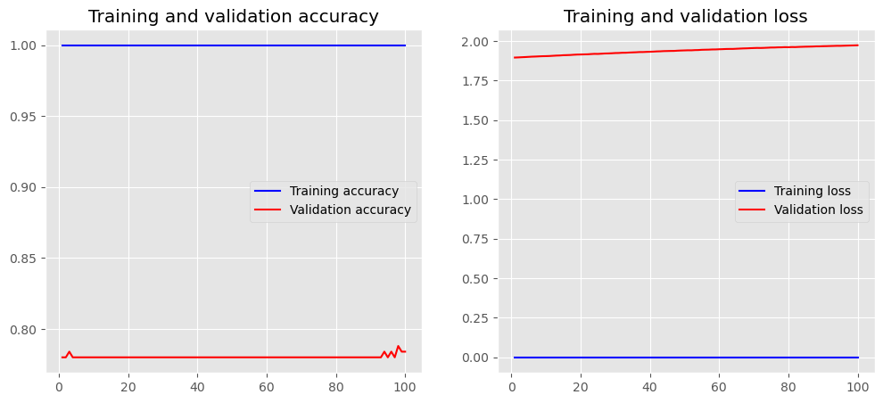
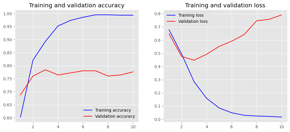
def plot_history(history):
    accuracy = history.history['accuracy']
    val_accuracy = history.history['val_accuracy']
    loss = history.history['loss']
    val_loss = history.history['val_loss']
    x = range(1, len(accuracy) + 1)


    plt.figure(figsize=(12, 5))
    plt.subplot(1, 2, 1)
    plt.plot(x, accuracy, 'b', label='Training accuracy')
    plt.plot(x, val_accuracy, 'r', label='Validation accuracy')
    plt.title('Training and validation accuracy')
    plt.legend()
    plt.subplot(1, 2, 2)
    plt.plot(x, loss, 'b', label='Training loss')
    plt.plot(x, val_loss, 'r', label='Validation loss')
    plt.title('Training and validation loss')
    plt.legend()


plot_history(history)
Output:
Word Embedding
Text is seen as a type of sequence data, much like the time series data found in financial or meteorological data. Now, We'll show you how to think of each word as a vector. Text can be vectorized in a variety of ways, which include:
- Each word is a vector that represents a word.
- Each character is a vector that represents a character.
- N-grams, or overlapping groupings of several subsequent words or characters in a text, are shown as a vector.
One Hot Encoding
One-hot encoding is the basic technique for turning a word into a vector, and it only entails taking a vector representing the vocabulary's length and adding 1 item for each word in the corpus.
Assuming each word has a place in the lexicon, we may create a vector for each one that is zero-filled everywhere save the word's designated location, which is set to one.
city = ['London', 'Berlin', 'Berlin', 'New York', 'London']
city
Output:

Use "LabelEncoder" to translate the list of cities into category integer values.
encode = LabelEncoder()
label_city = encode.fit_transform(city)
label_city
Output:

We must restructure the array since OneHotEncoder requires each category value to be in its own row. After that, we may use the encoder:
encode = OneHotEncoder(sparse=False)
label_city = label_city.reshape((5, 1))
encode.fit_transform(label_city)
Output:

Word Embeddings
In contrast to one-hot encoding, which is hardcoded, this approach encodes words as dense word vectors (also known as word embeddings) that are learned. In other words, word embeddings pack more data into fewer dimensions.
Remember that word embeddings don't reflect how a human would read the text; rather, they show the statistical organization of the language used in the corpus. Their goal is to translate semantic information into a geometric space. The embedding space is the term used to describe this geometric space.
The data must now be tokenized so the word embeddings may use it. We may use a few convenient techniques for text preprocessing and sequence preparation provided by Keras to get the text ready.
Starting with the Tokenizer utility class, which can vectorize a text corpus into a list of numbers, is a good place to start. The vocabulary words themselves serve as the keys to an encoding dictionary that uses each number to represent a value in the dictionary. The num words option, which determines the vocabulary's size, can be added. The words with the highest frequency (num_ words) will then be maintained.
token_ = Tokenizer(num_words=5000)
token_.fit_on_texts(sentences_train)


X_train = token_.texts_to_sequences(sent_train)
X_test = token_.texts_to_sequences(sent_test)


vocab_size = 1+ len(token_.word_index)   # We are Adding Because the 0th index is reserved


print(sent_train[2])
print(X_train[2])
Output:

for word in ['the', 'all','fan']:
    print('{}: {}'.format(word, token_.word_index[word]))
Output:

maxlength = 100


X_train = pad_sequences(X_train, padding='post', maxlen=maxlength)
X_test = pad_sequences(X_test, padding='post', maxlen=maxlength)


print(X_train[0, :])
Output:
Keras Embedding Layer
The Embedding Layer of Keras may now be used, which converts the integers that were previously computed into a dense vector of the embedding. The following parameters are necessary:
- input_dim: quantity of vocabulary
- output_dim: quantity of dense vector
- input_length: sequence’s length
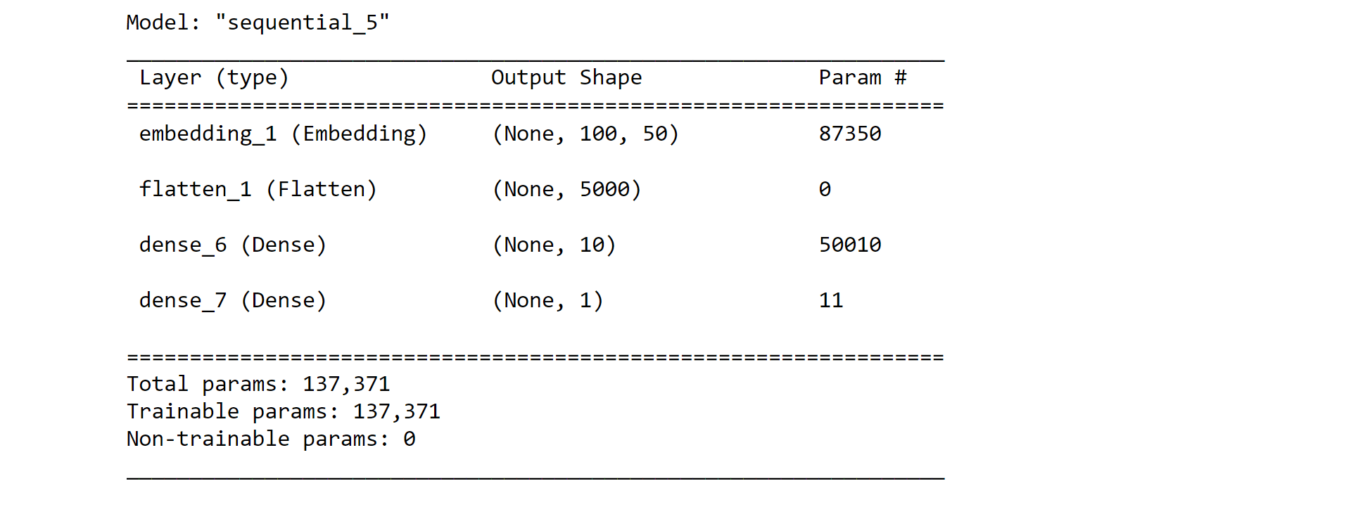
Now that we have the Embedding layer, we have a few alternatives. One approach would be to insert the embedding layer's output into a dense layer. To do this, we must insert a Flatten layer between them, which gets the sequential input ready for the Dense layer:
embedding_dim = 50


model_01 = Sequential()
model_01.add(layers.Embedding(input_dim=vocab_size,
                           output_dim=embedding_dim,
                           input_length=maxlength))
model_01.add(layers.Flatten())
model_01.add(layers.Dense(10, activation='relu'))
model_01.add(layers.Dense(1, activation='sigmoid'))
model_01.compile(optimizer='adam',
              loss='binary_crossentropy',
              metrics=['accuracy'])
model_01.summary()
Output:
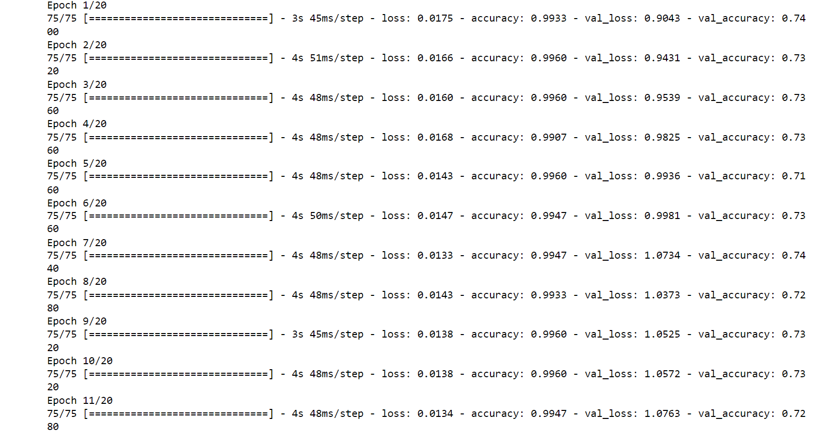
history = model_01.fit(X_train, y_train,
epochs=20,
verbose=True,
validation_data=(X_test, y_test),
batch_size=10)
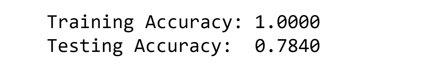
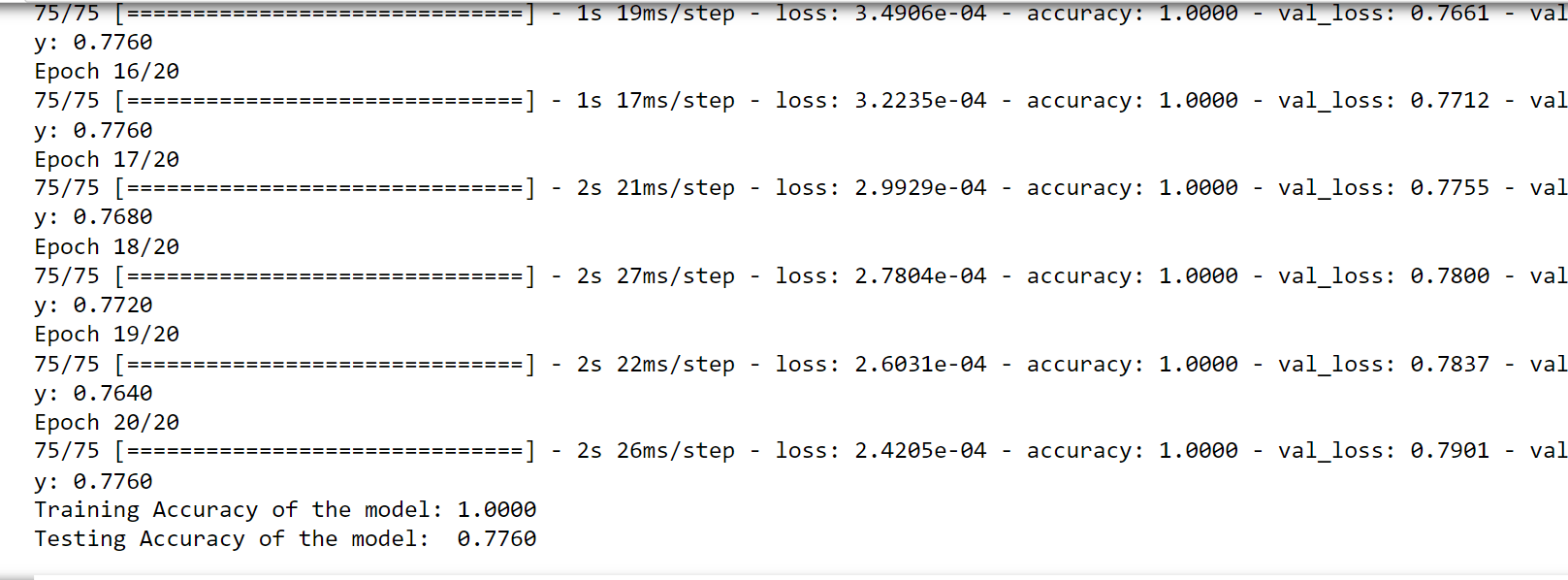
loss, accuracy = model_01.evaluate(X_train, y_train, verbose=False)
print("Training Accuracy of the model: {:.4f}".format(accuracy))
loss, accuracy = model_01.evaluate(X_test, y_test, verbose=False)
print("Testing Accuracy of the model: {:.4f}".format(accuracy))
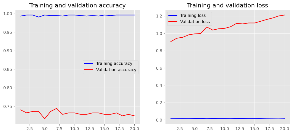
plot_history(history)
Output:
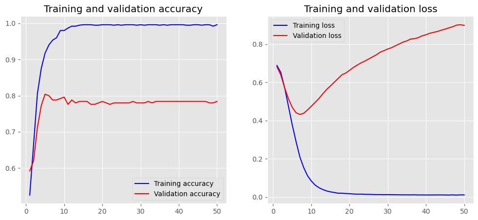
Global max/average pooling uses the highest/average value of all characteristics; however, in the alternative scenario, the size of the pool must be specified. Again, Keras has a layer of its own that can be added to the sequential model:
embedding_dim = 50
model_01 = Sequential()
model_01.add(layers.Embedding(input_dim=vocab_size,
output_dim=embedding_dim,
input_length=maxlength))
model_01.add(layers.GlobalMaxPool1D())
model_01.add(layers.Dense(10, activation='relu'))
model_01.add(layers.Dense(1, activation='sigmoid'))
model_01.compile(optimizer='adam',
loss='binary_crossentropy',
metrics=['accuracy'])
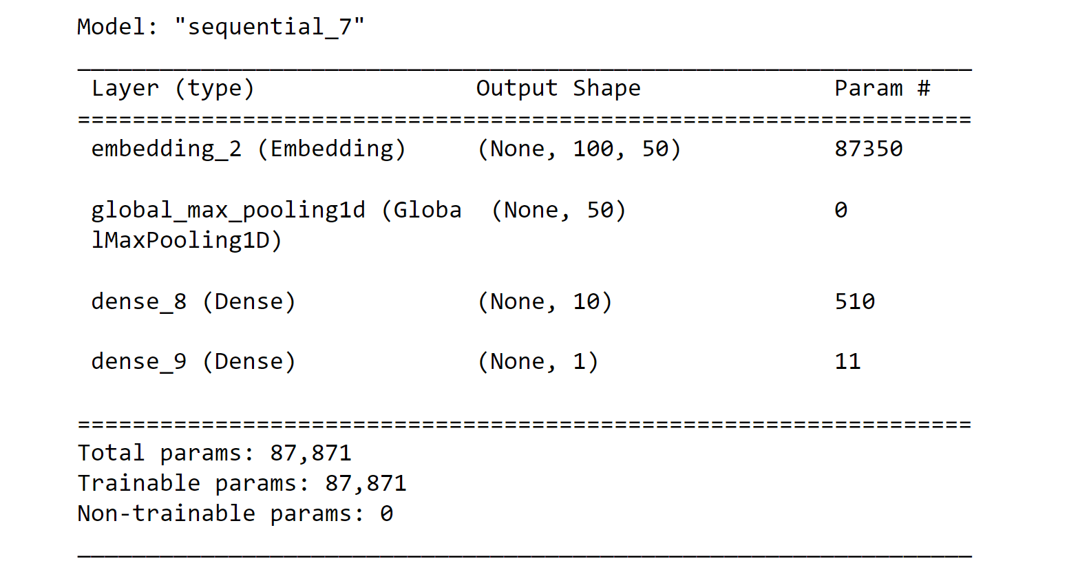
model_01.summary()
Output:
history = model_01.fit(X_train, y_train,
epochs=50,
verbose=False,
validation_data=(X_test, y_test),
batch_size=10)
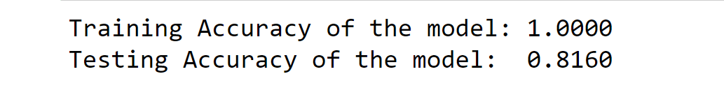
loss, accuracy = model_01.evaluate(X_train, y_train, verbose=False)
print("Training Accuracy of the model: {:.4f}".format(accuracy))
loss, accuracy = model_01.evaluate(X_test, y_test, verbose=False)
print("Testing Accuracy of the model: {:.4f}".format(accuracy))
plot_history(history)
Output:

CNN (Convolutional Neural Networks)
Convolutional neural networks, sometimes referred to as "convnets," are one of the most intriguing advancements in machine learning in recent years.
The ability to extract characteristics from pictures and use them in neural networks has revolutionized image categorization and computer vision. They are beneficial for sequence processing because they have the same qualities that make them valuable for image processing. A CNN may be viewed as a customized neural network that can recognize particular patterns.
Convolutional layers are the hidden layers of a CNN. A computer must deal with a two-dimensional numeric matrix while thinking of images. Thus we must find a mechanism to identify characteristics in this matrix. These convolutional layers are such a unique tool because they can recognize edges, corners, and other textures. The convolutional layer is made up of many filters that may track certain characteristics as they move across the picture.
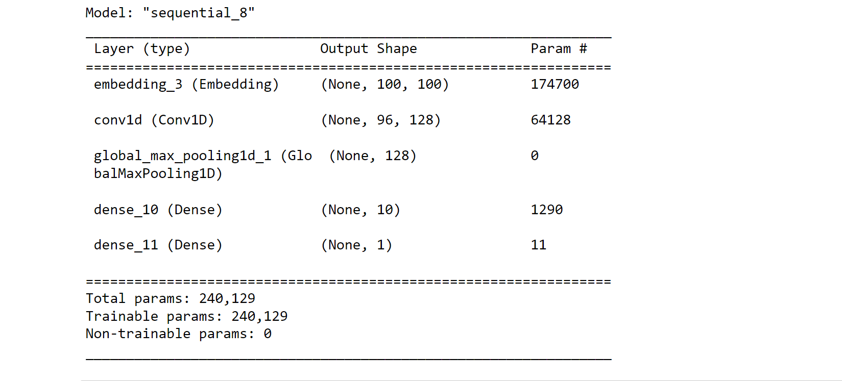
embedding_dim = 100


model_02 = Sequential()
model_02.add(layers.Embedding(vocab_size, embedding_dim, input_length=maxlength))
model_02.add(layers.Conv1D(128, 5, activation='relu'))
model_02.add(layers.GlobalMaxPooling1D())
model_02.add(layers.Dense(10, activation='relu'))
model_02.add(layers.Dense(1, activation='sigmoid'))
model_02.compile(optimizer='adam',
              loss='binary_crossentropy',
              metrics=['accuracy'])
model_02.summary()
Output:
history = model_02.fit(X_train, y_train,
epochs=10,
verbose=False,
validation_data=(X_test, y_test),
batch_size=10)
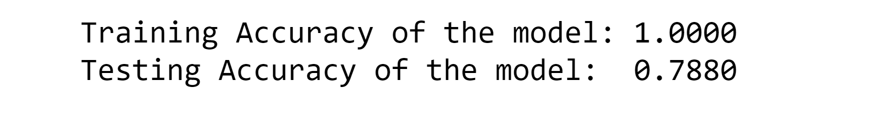
loss, accuracy = model_02.evaluate(X_train, y_train, verbose=False)
print("Training Accuracy of the model: {:.4f}".format(accuracy))
loss, accuracy = model_02.evaluate(X_test, y_test, verbose=False)
print("Testing Accuracy of the model: {:.4f}".format(accuracy))
plot_history(history)
Output:
Hyperparameters Optimization
Hyperparameter optimization is the process of choosing the best set of hyperparameters for a machine-learning model. Hyperparameters are values that are set before training a model, and they can greatly impact the performance of the model.
Even with simpler models, as we saw in the ones we have used thus far, you have a wide range of factors to adjust and select from. They are referred to as hyperparameters. The most time-consuming aspect of machine learning is this, and alas, there are no ready-made solutions that work for everyone.
Grid search is a well-liked technique for hyperparameter optimization. With the use of parameter lists, this approach runs the model with every possible combination of parameters. It is the complete method, but it also requires a lot of processing power. Another popular method is random search, which you'll see in action below. It just uses random parameter combinations.
We must use the KerasClassifier, a wrapper for the scikit-learn API, in order to utilize random search with Keras. We may use this wrapper to access the different Scikit-Learn utilities, including cross-validation. We require the class known as RandomizedSearchCV, which does cross-validation with random search. Cross-validation is a technique for model validation that divides the entire data set into many training and testing data sets.
Cross-validation comes in a variety of forms. K-fold cross-validation is one kind. In this kind, the data set is divided into k equal-sized sets, one of which is utilized for training and the other for testing. This allows you to do k distinct runs, with each partition serving as a testing set once throughout each run. Therefore, the model assessment is more accurate, but each testing set is smaller the greater the value of k.
def create_model(num_filters, kernel_size, vocab_size, embedding_dim, maxlen):
model_03 = Sequential()
model_03.add(layers.Embedding(vocab_size, embedding_dim, input_length=maxlength))
model_03.add(layers.Conv1D(num_filters, kernel_size, activation='relu'))
model_03.add(layers.GlobalMaxPooling1D())
model_03.add(layers.Dense(10, activation='relu'))
model_03.add(layers.Dense(1, activation='sigmoid'))
model_03.compile(optimizer='adam',
metrics=['accuracy'],
loss='binary_crossentropy')
return model_03
grid_Param= dict(vocab_size=[5000],
kernel_size=[3, 5, 7],
num_filters=[32, 64, 128],
embedding_dim=[50],
maxlen=[100]
)
# Settings for the hyperparameter optimization
using_epochs = 20
using_embedding_dim = 50
using_maxlength = 100
using_output_file = 'output.txt'
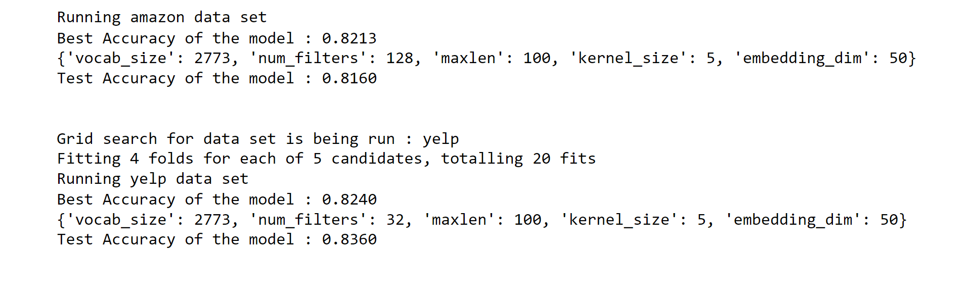
# Running grid search for every source ( amazon, imdb, yelp)
for source, frame in af.groupby('source'):
print(Grid search for data set is being run :', source)
sent = af['sentence'].values
y = af['label'].values
# Splitting the dataset into Train -Test Dataset
sent_train, sent_test, y_train, y_test = train_test_split(
sent, y, random_state=1000,test_size=0.25)
# Tokenizing words
token_ = Tokenizer(num_words=5000)
token_.fit_on_texts(sent_train)
X_train = token_.texts_to_sequences(sent_train)
X_test = token_.texts_to_sequences(sent_test)
# We are adding 1 because the 0th index is reserved.
vocab_size = len(token_.word_index) + 1
# Pad sequences along with 0
X_train = pad_sequences(X_train, padding='post', maxlen=maxlength)
X_test = pad_sequences(X_test, padding='post', maxlen=maxlength)
# Parameter grid for grid search
grid_Param= dict(num_filters=[32, 64, 128],
kernel_size=[3, 5, 7],
embedding_dim=[using_embedding_dim],
vocab_size=[vocab_size],
maxlen=[using_maxlength])
model_X = KerasClassifier(build_fn=create_model,
batch_size=10,epochs=using_epochs,
verbose=False)
grid = RandomizedSearchCV(estimator=model_X, param_distributions=grid_Param,
cv=4, verbose=1, n_iter=5)
grid_result = grid.fit(X_train, y_train)
# Evaluating Test Dataset
accuracy_of_test = grid.score(X_test, y_test)
s = ('Running {} data set\nBest Accuracy of the model : '
'{:.4f}\n{}\nTest Accuracy of the model : {:.4f}\n\n')
output_string = s.format(
source,
grid_result.best_score_,
grid_result.best_params_,
accuracy_of_test )
print(output_string)
Output:

Conclusion
In conclusion, text classification is an important task in NLP and machine learning. It can be performed using machine learning by following the steps of collecting data, preprocessing, feature extraction, model selection, training, evaluation and deploying it to production. With the use of machine learning, text classification can be performed with high accuracy and speed, making it useful in various applications.