Decision Trees in Machine Learning

Introduction to Decision Trees

Decision trees are one of the most powerful classification algorithm that falls under supervised learning-based algorithms. It is used as a tool for making predictions and can be incorporated in different fields. With the help of decision trees, the data-set can be divided in different ways on the basis of different conditions.

The main entities of a decision tree are the decision nodes and the leaves. The decision nodes are the ones where the data gets fragmented, whereas the leaves are one where we get the output. The concept of the decision tree can be used for both regressions as well as the classification model.

A decision tree is a tree-like arrangement of a flowchart. An example of a decision tree is given below:

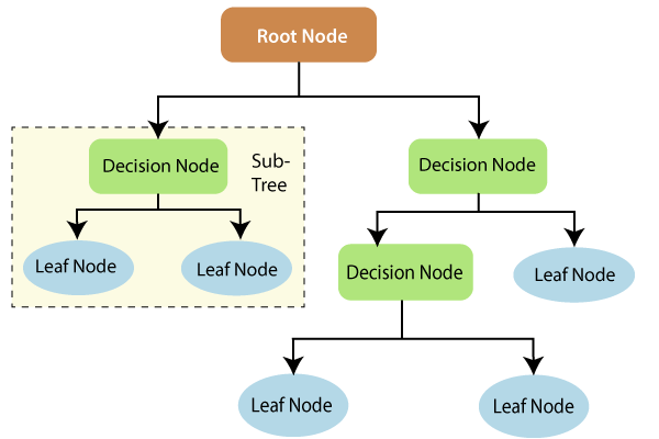
From the given image, some of the following terminologies used with Decision Trees are discussed below:

Root Node: It is the very first node, or we can call it as a parent node. It denotes the whole population and gets split into two or more Decision nodes based on the feature value.

Decision Node: Splitting of a sub-node into more no. of sub-nodes, is called a decision node.

Leaf Node: These are the terminal nodes, as it cannot get split further. 

Sub-Tree: A branch is a subdivision of a complete tree.

Advantages of Decision Trees:

1. Since it does not require any prerequisite statistical knowledge for reading and interpreting the data, it makes it much easier even for the users who belongs from a non-technical background to understand the output.
2. It works fastest, finding the most significant variables as well as the relationship among the variables. New variables can be created with the help of a decision tree based on its prediction power.
3. Feature selection and variable screening are correctly accomplished by the decision tree.
4. It requires very little effort to prepare the data by the users.
5. It does not get influenced by outliers and missing values, so it does not need cleaning of the data.
6. It is not concerned with the data type, which means it can handle both categorical as well as numerical data.
7. It is a non-parametric model.
8. The performance does not get affected by the non-linear relation between the parameters.

Disadvantages of Decision Trees:

1. One of the major disadvantage of the decision tree is to handle the issue of Overfitting.
2. It is difficult to categories the variables in the different category while working with the continuous variables for a long time, as it may lead to loss of information by the tree.
3. Decision trees are changeable in nature, i.e., a small change in the data can totally change the generated data. To resolve such issues boosting and bagging is needed to be done.
4. For the dominated classes, the decision tree learners build biased trees.
5. In comparison with the other algorithm, it results in low predicted accuracy.
6. The calculations become very complex, with so many class records.

Now we will see how a Decision Tree classifier differentiates two different classes into two different categories, and then we will compare its results with the previous classification models using the same dataset as we used in the previous model i.e., Social_Network_Ads. We will again start with importing the libraries and performing data pre-processing as done in the earlier models.

# Import the libraries
import numpy as np
import matplotlib.pyplot as plt
import pandas as pd 

# Import the dataset
dataset = pd.read_csv('Social_Network_Ads.csv')
X = dataset.iloc[:, [2, 3]].values
y = dataset.iloc[:, 4].values 

# Split the dataset into the Training set and Test set
from sklearn.model_selection import train_test_split
X_train, X_test, y_train, y_test = train_test_split(X, y, test_size = 0.25, random_state = 0)

# Feature Scaling
from sklearn.preprocessing import StandardScaler
sc = StandardScaler()
X_train = sc.fit_transform(X_train)
X_test = sc.transform(X_test) 

After we are done with the pre-processing step, we will fit the decision tree classifier to the training set. Firstly we will import the DecisionTree library from scikit learn and create its variable naming it as a classifier, which is the object of a decision tree.

We will pass two arguments that are; criterion and the random_state, which is equal to 0. For the criterion, the default parameter is “gini”, but we will take the decision tree based on entropy because the most common decision trees are based on entropy, for example, maximum entropy for NLP.

And then, we will fit the classifier to X_train and Y_train, as usual, to help the classifier in learning the correlation between the X_train and Y_train.

# Fit Decision Tree Classifier to the Training set
from sklearn.tree import DecisionTreeClassifier
classifier = DecisionTreeClassifier(criterion = 'entropy', random_state = 0)
classifier.fit(X_train, y_train) 

Next, we will predict the observations, and for that, we will create a variable named y_pred, which is the vector of prediction containing the predictions of test_set results. And then, we will make the confusion matrix carried out in the same way as done in previous models.

# Predicting the Test set results
y_pred = classifier.predict(X_test)
# Making the Confusion Matrix
from sklearn.metrics import confusion_matrix
cm = confusion_matrix(y_test, y_pred) 

Output:

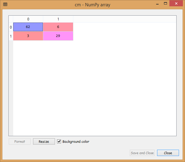
From the output image given above, it can be seen that we have nine incorrect predictions on the test_set.

In the end, we will visualize the training set and test set results as we did in prior models, simply by plotting a graph that will separate out the region that predicts the users who will purchase the SUV from the region predicting those users who will not buy the SUV.

Visualizing the Training Set Results:

To visualize the training set results, we will plot a graph where the decision tree classifier is going to predict Yes for the users who will purchase the SUV and No for the users who will buy the SUV, the same way as we did in the previous models. 

# Visualizing the Training set results
 from matplotlib.colors import ListedColormap
 X_set, y_set = X_train, y_train
 X1, X2 = np.meshgrid(np.arange(start = X_set[:, 0].min() - 1, stop = X_set[:, 0].max() + 1, step = 0.01),
                      np.arange(start = X_set[:, 1].min() - 1, stop = X_set[:, 1].max() + 1, step = 0.01)) 
 plt.contourf(X1, X2, classifier.predict(np.array([X1.ravel(), X2.ravel()]).T).reshape(X1.shape),
              alpha = 0.75, cmap = ListedColormap(('red', 'green')))
 plt.xlim(X1.min(), X1.max())
 plt.ylim(X2.min(), X2.max())
 for i, j in enumerate(np.unique(y_set)):
     plt.scatter(X_set[y_set == j, 0], X_set[y_set == j, 1],
                 c = ListedColormap(('red', 'green'))(i), label = j)
 plt.title('Decision Tree Classification (Training set)')
 plt.xlabel('Age')
 plt.ylabel('Estimated Salary')
 plt.legend()
 plt.show() 

Output:

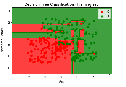
From the output image given above, it can be seen that here, the prediction boundary comprise of only horizontal and vertical lines. It is performing the split based on some conditions on independent variables, which are age and the estimated salary.

It is trying to grab every single user falling in the true set. It doesn’t want to skip any user, even the red user in the green region or vice versa. And as it is trying to catch every single user, it is a case of Overfitting.

Visualizing the Test Set Results:

We will visualize the Test Set results in the same way as we did earlier.

# Visualizing the Test set results
 from matplotlib.colors import ListedColormap
 X_set, y_set = X_test, y_test
 X1, X2 = np.meshgrid(np.arange(start = X_set[:, 0].min() - 1, stop = X_set[:, 0].max() + 1, step = 0.01),
                      np.arange(start = X_set[:, 1].min() - 1, stop = X_set[:, 1].max() + 1, step = 0.01))
 plt.contourf(X1, X2, classifier.predict(np.array([X1.ravel(), X2.ravel()]).T).reshape(X1.shape),
              alpha = 0.75, cmap = ListedColormap(('red', 'green'))) 
 plt.xlim(X1.min(), X1.max())
 plt.ylim(X2.min(), X2.max())
 for i, j in enumerate(np.unique(y_set)):
     plt.scatter(X_set[y_set == j, 0], X_set[y_set == j, 1],
                 c = ListedColormap(('red', 'green'))(i), label = j)
 plt.title('Decision Tree Classification (Test set)') 
 plt.xlabel('Age')
 plt.ylabel('Estimated Salary')
 plt.legend()
 plt.show() 

Output:

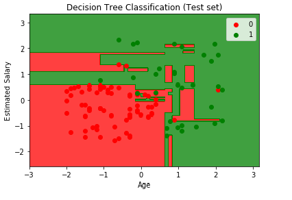
It can be seen from the above image, that for some new observations, it is catching red users in green region and vice versa. But we can say it did a good job in calculating all the 9 incorrect predictions. This is only 1 prediction tree, but you can simply imagine what will be the result if you evaluate about 500 or even more decision trees, which is a case of Random Forest and that we will learn in next chapter.