Feature Extraction in Machine Learning

With the advancement of technology in the databases, everyone can store a vast amount of data with hundreds of thousands of features these days. Features contain information about the dependent or target variable. So, we may assume that a more significant number of features means more details on the target variable. But this may not be the case all the time. Because the datasets consist of relevant, irrelevant, and correlated features. While building a machine learning model with datasets which consist of a massive number of features, it becomes complicated for us to visualize and analyze. It also consumes a lot of time and memory, increasing the model's time and space complexity. Sometimes, the model may perform poorly on the testing data because of the irrelevant features in the dataset.

So, here comes the importance of Feature Reduction in Machine Learning. Feature reduction is a data pre-processing technique.

Feature reduction is reducing the number of features available in the dataset. This feature reduction is classified into the following types. They are,

• Feature Selection
• Feature Extraction

In this tutorial, let us discuss about Feature extraction in detail.

Note:

One of the important terms that are often used in Machine Learning is dimensionality.

Dimensionality is equal to the number of features in a dataset.

A dataset with three features can be visualized in a three-dimensional plane.

Feature reduction is also known as dimensionality reduction.

Feature Extraction:

Feature extraction is taking/considering the features from the given dataset and mapping it to a lower dimensional set in which each feature is obtained as a function of the original feature set.

Let us assume that initially, there are ‘m’ number of features in the original dataset. Now the number features say ‘n’ in the lower dimensional set must be less than the value of ‘m’.

In general, feature extraction is the process of establishing a relation among several features to get a new feature. 

For example, let us consider an IPL dataset which consists of three features MatchesPlayed, RunsScored, and BallsFaced. Now the value of m is three. Here we can establish a relation between RunsScored, BallsFaced to obtain a new feature known as StrikeRate, which is given by the formula,

StrikeRate = RunsScored/BallsFaced   

Now the number of features has become two (i.e., n=2), which is less than m.

Some of the characteristics that we expect from the new features are,

• When we establish a relation among several features, the derived new feature should be uncorrelated and cannot be reduced further.
• The new features must have larger variances because you want the features to be able to distinguish between different instances.

Advantages of Feature Extraction:

• Improvement in accuracy of our model
• No redundancy in the data
• Better visualization of data
• Reduces the risk of overfitting
• Increase in speed of training our model by reducing time complexity
• Reduction in the computation of our model.
• Memory management

Practical Applications of Feature Extraction:

• Feature extraction is commonly used in Machine Learning while dealing with a dataset which consists of a massive number of features.
• In Natural language Processing (NLP), feature extraction is used to identify specific keywords based on their frequency of occurrence in a sentence or a file.
• Feature extraction is also used in the field of Image Processing in order to detect some features of a particular image.

Principal Component Analysis:

Principal Component Analysis, shortly PCA, plays a key role in feature extraction.

In PCA, we take our original dataset as input and try to establish a relation among certain features or combine certain features to create a new feature ensuring that no information is lost during the process.

In PCA, our data is projected into a set of orthogonal axes and drawn, some principal components and select one with minor information loss. Let us understand this concept with an example.

Consider a dataset with two features (Gene1, Gene2) and scatter the data points in a two-dimensional plane.

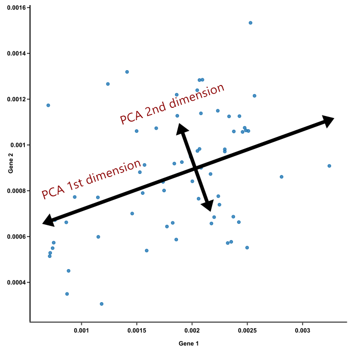
Now let us try to draw two components in the graph (you can draw any number of components) and project these datapoints onto the components. We select the best component which has lower information loss.

In PCA, all the principal components drawn will be perpendicular to each other, as shown in the above figure.

Implementation of PCA on a sklearn Dataset:

The steps involved in implementing PCA in Machine Learning are

• Importing the required libraries
• Loading the dataset
• Analyzing the dataset
• Creating a dataframe
• Scaling all the values in all columns
• Transforming all the columns
• Implementing PCA
• Visualization

Code:

#importing required libraries
import pandas as pd
import numpy as np
import matplotlib.pyplot as plt
import seaborn as sns
#loading the data
from sklearn.datasets import load_wine
wine = load_wine()
#analyzing the dataset
wine.keys() 

Output:

dict_keys(['data', 'target', 'frame', 'target_names', 'DESCR', 'feature_names'])

Input:

#creating a dataframe
df = pd.DataFrame(wine['data'],columns = wine['feature_names'])	
df.head(10)

Output:

	alcohol	malic_acid	ash	alcalinity_of_ash	magnesium	total_phenols	flavanoids	nonflavanoid_phenols	proanthocyanins	color_intensity	hue	od280/od315_of_diluted_wines	proline
0	14.23	1.71	2.43	15.6	127.0	2.80	3.06	0.28	2.29	5.64	1.04	3.92	1065.0
1	13.20	1.78	2.14	11.2	100.0	2.65	2.76	0.26	1.28	4.38	1.05	3.40	1050.0
2	13.16	2.36	2.67	18.6	101.0	2.80	3.24	0.30	2.81	5.68	1.03	3.17	1185.0
3	14.37	1.95	2.50	16.8	113.0	3.85	3.49	0.24	2.18	7.80	0.86	3.45	1480.0
4	13.24	2.59	2.87	21.0	118.0	2.80	2.69	0.39	1.82	4.32	1.04	2.93	735.0
5	14.20	1.76	2.45	15.2	112.0	3.27	3.39	0.34	1.97	6.75	1.05	2.85	1450.0
6	14.39	1.87	2.45	14.6	96.0	2.50	2.52	0.30	1.98	5.25	1.02	3.58	1290.0
7	14.06	2.15	2.61	17.6	121.0	2.60	2.51	0.31	1.25	5.05	1.06	3.58	1295.0
8	14.83	1.64	2.17	14.0	97.0	2.80	2.98	0.29	1.98	5.20	1.08	2.85	1045.0
9	13.86	1.35	2.27	16.0	98.0	2.98	3.15	0.22	1.85	7.22	1.01	3.55	1045.0

Input:

#scaling
from sklearn.preprocessing import StandardScaler
scaler = StandardScaler()
scaler.fit(df)
#tranforming the values
scaled_data = scaler.transform(df)
#implementing PCA
from sklearn.decomposition import PCA
pca = PCA(n_components=2)
pca.fit(scaled_data)

Output:

PCA(n_components=2)

Input:

x_pca = pca.transform(scaled_data)
#identifying the number of columns
print("The shape of original dataset:",scaled_data.shape)
print("The shape of dataset after implementing PCA:",x_pca.shape)

Output:

The shape of original dataset: (178, 13)
The shape of dataset after implementing PCA: (178, 2)

Implementing PCA has reduced the number of features from 13 to 2.

Input:

#visualization
plt.scatter(x_pca[:,0],x_pca[:,1],c = wine['target'])
plt.xlabel("First Principal Component")
plt.ylabel("Second Principal Component")
plt.show()

Output:

Here comes to the end of implementing PCA. Now we can use any machine learning classification algorithm to train the model.