FCFS Scheduling in OS

FCFS: First Come First Serve Scheduling in OS

FCFS is a non-preemptive and preemptive scheduling algorithm that is easy to understand and use. In this, the process which reaches first is executed first, or in other words, the process which requests first for a CPU gets the CPU first.

Example of FCFS: buying tickets at the ticket counter.

FCFS is similar to the FIFO queue data structure. In FCFS, the element which is added in the queue first will leave first.

FCFS is used in Batch Operating Systems.

Characteristics of FCFS Scheduling

The characteristics of FCFS Scheduling are:

1. FCFS is simple to use and implement.
2. In FCFS, jobs are executed in a First-come First-serve (FCFS) manner.
3. FCFS supports both preemptive as well as non-preemptive scheduling algorithm.
4. FCFS is poor in performance due to high waiting times.

Advantages of FCFS

The advantages of FCFS are:

1. Easy to program
2. First come, first serve
3. Simple scheduling algorithm.

Disadvantages of FCFS

1. Because of non-preemptive nature, the problem of starvation arises.
2. More Average waiting time.
3. Due to its simplicity, FCFS is not effective.
4. FCFS is not the ideal scheduling for the time-sharing system.
5. FCFS is a Non-Preemptive Scheduling algorithm, so allocating the CPU to a process will never release the CPU until it completes its execution.
6. In FCFS, it is not possible to use the resources in a parallel manner, which causes the convoy effect, so the resource utilization is poor in FCFS.

What is Convoy Effect

In FCFS, Convoy Effect is a condition that arises in the FCFS Scheduling algorithm when one process holds the CPU for a long time, and another process can get the CPU only when the process holding the CPU finishes its execution. Due to this, resource utilization is poor and also affects the performance of the operating system.

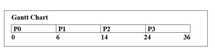
Example of FCFS Scheduling

In the following example, we have 4 processes with process ID P0, P1, P2, and P3. The arrival time of P0 is 0, P1 is 1, P2 is 2, and P3 is 3. The arrival time and burst time of the processes are given in the following table.

The waiting time and Turnaround time are calculated with the help of the following formula.

         Waiting Time = Turnaround time – Burst Time

          Turnaround Time = Completion time – Arrival time 

Process ID	Arrival Time	Burst Time	Completion Time	Turnaround Time	Waiting Time
P0	0	6	6	6	0
P1	1	8	14	13	5
P2	2	10	24	22	12
P3	3	12	36	33	21

Average Waiting Time = 0+5+12+21/4

                                         = 38/4

                                          = 9.5 ms

Average Turnaround Time = 6+13+22+33/4

                                              =74/4

                                               = 18.5 ms

Related Posts:

• Deadlock Prevention in Operating System
• SCAN Disk Scheduling Algorithm
• Resource Allocation Graph in Operating System
• Fixed Partitioning in Operating System
• Disk Scheduling Algorithms
• Difference between Multi-programming and Multitasking
• Deadlock Detection and Recovery
• Lock Variable Mechanism | Operating System
• Process Synchronization | Operating System
• Round-Robin Scheduling Algorithm in OS