Array Formula in Excel
How to use Array Formula in Excel?
By default, Excel consists of various formulas for calculating the data. Among various formulas, the Array formula is a powerful one that is used to calculate tough or complicated calculations. Array formulas are known as the CSE formula pressing “Ctrl+Shift+Enter” to be used to enter the data. The variation purpose of the array formula includes Counting characters and the Sum of the nth value and numbers in the range of cells. Array formula in Excel performs two types of calculations such as:
- Performing multiple calculations to display the single result
- Perform calculations to generate multiple results.
Usually, the array formula is used to replace multiple formulas to get the result quickly and saves time. It generates multiple results, and it processes multiple values in a single time based on the given conditions. Sometimes it returns multiple values. Hence the result obtained is also in the array format.
Array in Excel
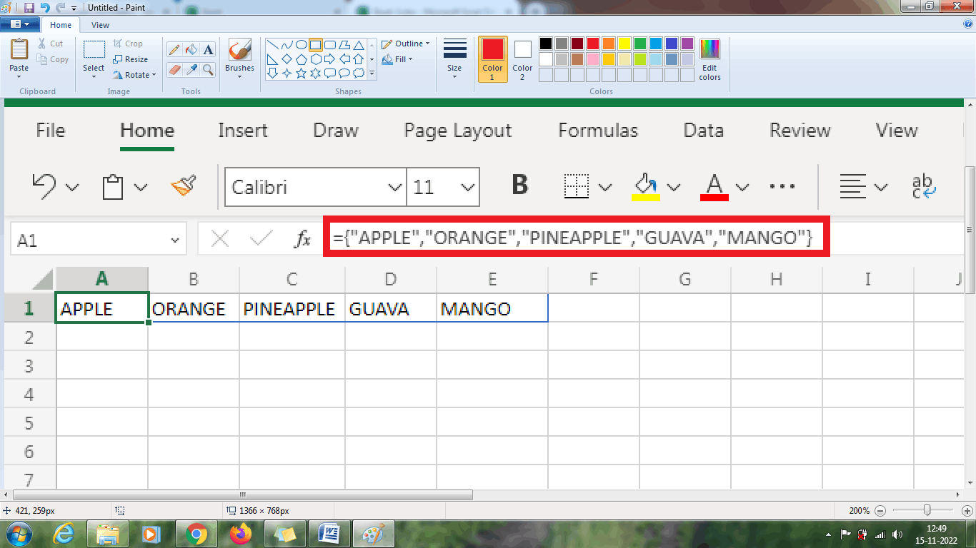
The array is defined as a collection of items. Items include numbers or alphabets in a single row, column, or multiple rows and columns. Here is an example to illustrate the data using the array formula. The steps to be followed are,
Step 1: To enter the five fruits' names in the cell, select the cell range from A1:E1.
Step 2: Type the data proceeded by an equal sign as = {"APPLE", "ORANGE", "PINEAPPLE", "GUAVA", "MANGO”}
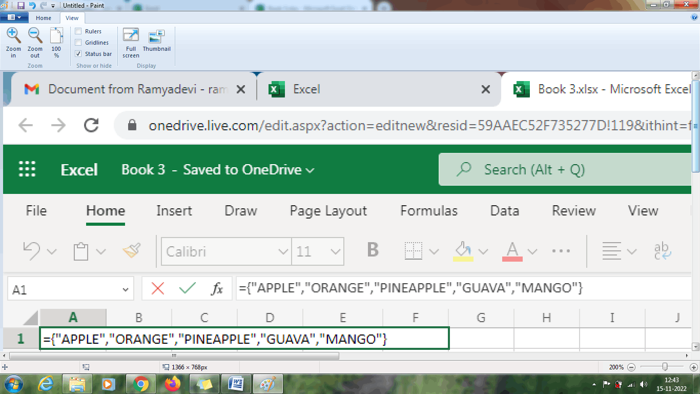
Step 3: Press Enter key or click CTRL+SHIFT+ENTER. The result will be displayed in the cell as shown in the image.
Example 1: The data contains the stationery items with the quantity of how much it is sold and the amount. How to calculate the total of all sales?
The first method to calculate the total of all sales using the normal Excel formula as follows,
Step 1: Enter the data in the spreadsheet from the row and column range A1:C7.
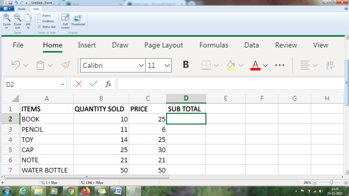
Step 2: To find the subtotal enter the formula in the cell D2 as =B2*C2. Drag the formula down to fill the entire column from range D3:D7. The result will be displayed in cell D2.
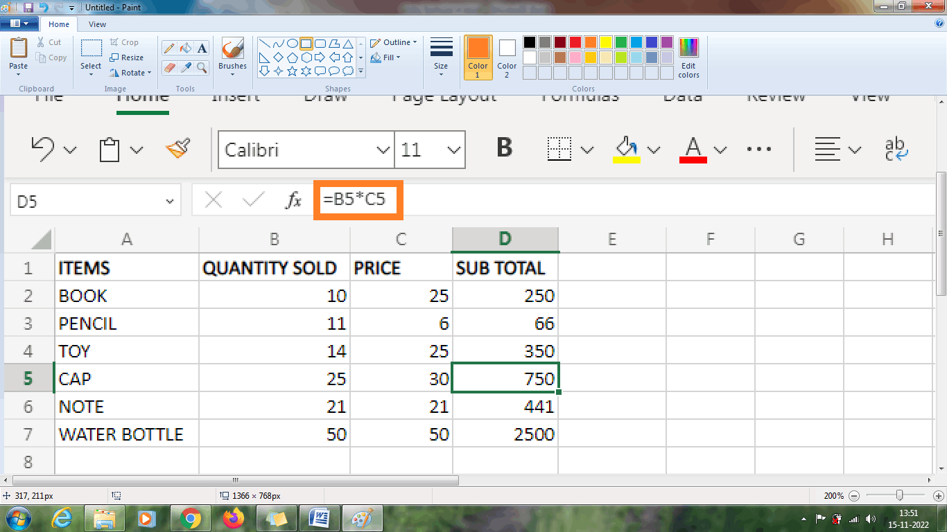
Step 3: Enter the formula in cell D8 as = SUM (D2:D7) to calculate the sub-total.
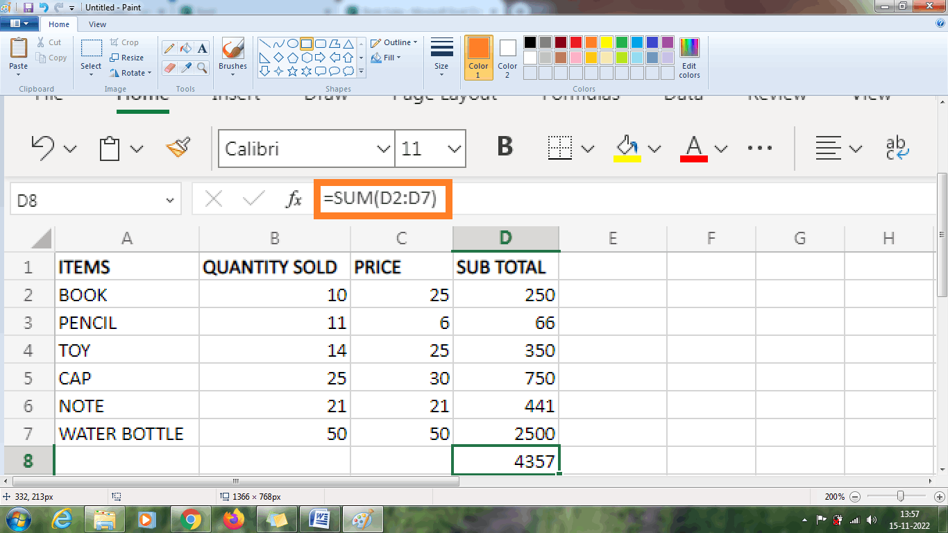
From the above worksheet, the subtotal is calculated using the formula.
An alternative method to calculate the “total sales” using the array formula is as follows,
Step 1: Enter the formula in the cell D8 as =SUM (B2:B7*C2:C7)
Step 2: Press Enter key or click CTRL+SHIFT+ENTER using the keyboard shortcut.
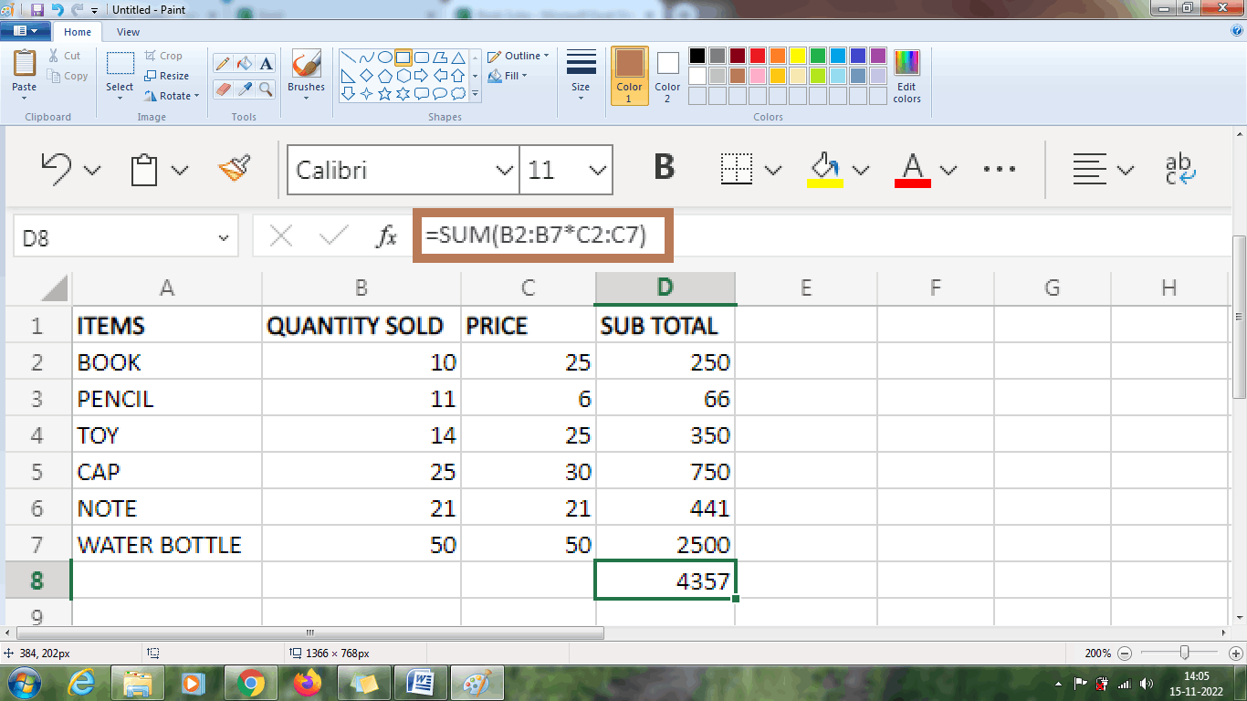
From the above worksheet, the result displayed in cell D8 using the array formula is similar to the previous concept using the normal Excel formula. It shows that an array is a powerful formula that saves time. Hence from the above two methods, the array can calculate more than one calculation and returns a single result based on the data.
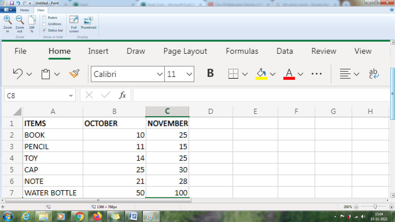
Example 2: How to get the result in a single-cell array formula from the given data?
The data contains the list of items, and sales for two months are described. How to calculate the maximum sales in the given data?
Step 1: Enter the data in the spreadsheet in the respective row and column, A1:C7.
Usually, in the general method to calculate the maximum sales, the formula used is =C2-B2. It is entered in the new cell D1 and drags the formula downwards. After calculating, sum the data which is present in the column range D2:D7.Similarly, an alternative method is calculating the maximum sale using an array formula.
Step 2: Enter the formula in the cell C8 as =MAX (C2:C6-B2:B6). The result is displayed in the cell.
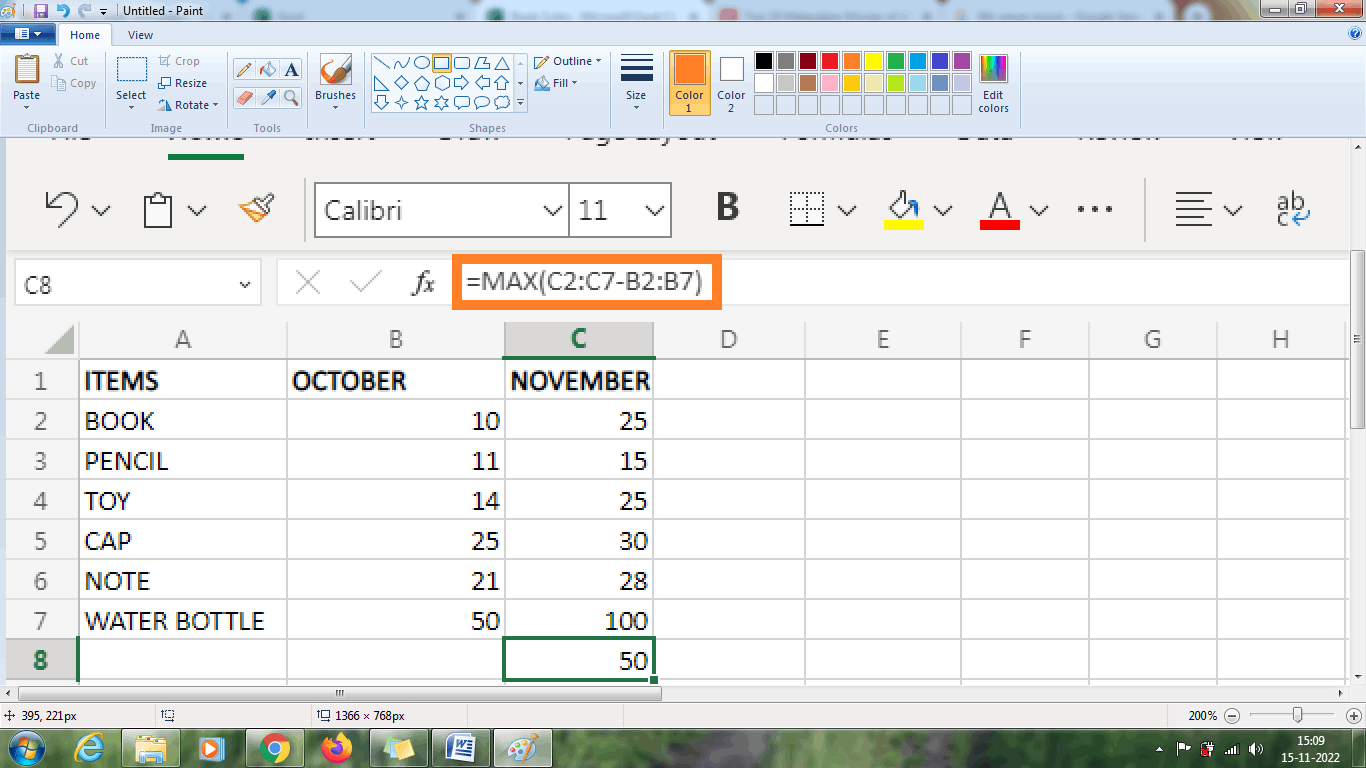
The above worksheet shows the result in cell C8 as 50, which is the maximum sale increase for the given data without the need for the new column.
Example 2.1: How to get the result in a multi-cell array formula from the given data?
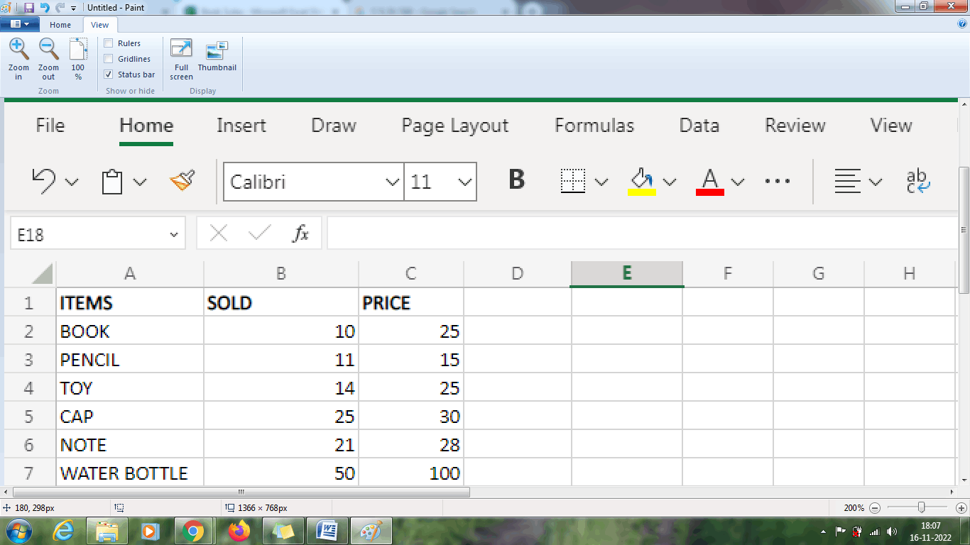
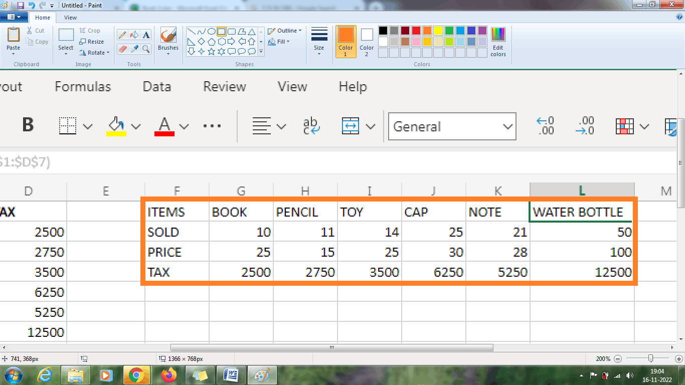
The given data consists of product, price, and quantity of product sold. Suppose the user needs to pay a 10% tax for each sale. To calculate the tax amount for each product, the array formula is used to calculate the result.
1. Enter the data in the spreadsheet from the row and column range, namely A1:C7
2. To calculate the tax, select the cell range from D2:D6 and enter the formula in the formula bar as =B2:B6*C2:C6*0.1
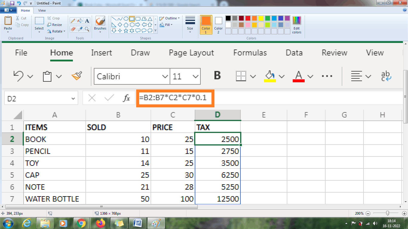
3. The result will be displayed in the above image, which calculates the result for the selected cell using the array formula.
Example 3: How to convert the array into a multi-cell array?
To convert the array into a multi-cell array, the transpose function transposes the data in the table.
Here, the data in the row are converted to columns using the transpose function. The steps to be followed are,
1. Enter the data in the respective row and column.
2. Select the range of empty cells to display the transposed data. An equal number of rows and columns is selected to display the data. Here 7 columns and 4 rows are selected called F1:L4.
3. In the formula, bar enters the formula as =TRANSPOSE ($A$1:$D$7)
4. Press CTRL+SHIFT+ENTER or press Enter key. The transposed data will display in the new location.
The following steps above convert the array data into transposed data using the TRANSPOSE function.
Array constants in Excel
The values in the array constant won't modify if the formula is copied to other values or cells. In Excel, the array constants are sub-divided into the following types,
- Horizontal array constant
- Vertical array constant
- A two-dimensional array is constant.
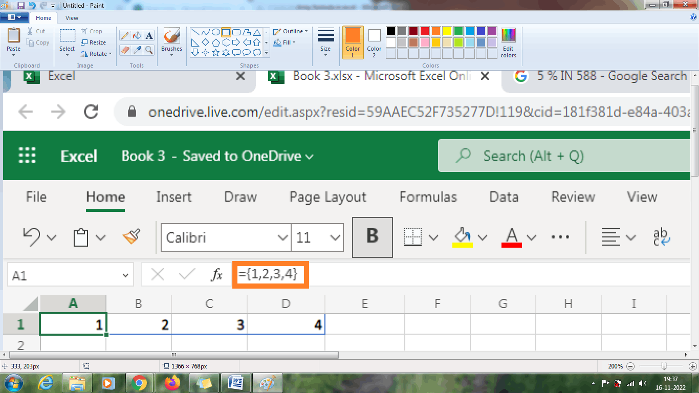
Horizontal array constant
The horizontal array is represented in the row. The data are represented using commas and braces at the start and end of the data.
The steps to be followed to represent the horizontal array are,
Step 1: Select the empty cells where the data needs to be displayed. Here the ranges selected are A1:E5.
Step 2: Type the formula in the formula bar as = {1, 2, 3, 4}
Step 3: Press CTRL+SHIFT+ENTER or press Enter key. The data will be displayed in the selected cell as follows,
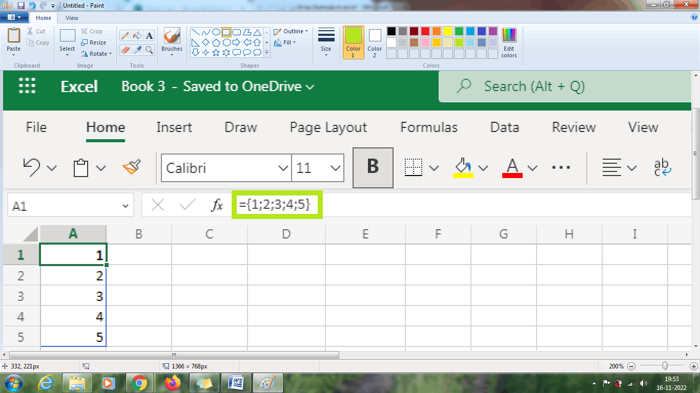
Vertical array constant
The vertical array is represented in the column. The data are represented using semicolons and braces at the start and end of the data.
The steps to be followed to represent the vertical array are,
Step 1: Select the empty cells where the data needs to be displayed. Here the column ranges selected are A1:A5.
Step 2: Type the formula in the formula bar as = {1; 2; 3; 4; 5}
Step 3: Press CTRL+SHIFT+ENTER or press Enter key. The data will be displayed in the selected cell as follows,
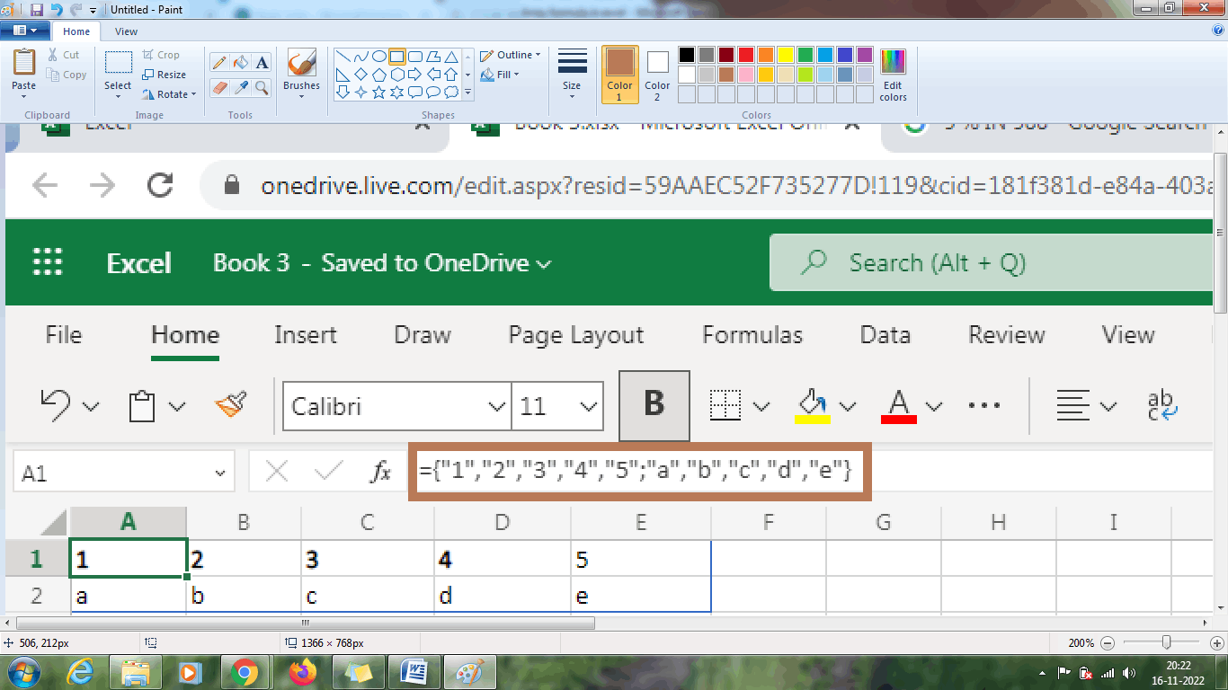
Two-dimensional Array Constant
The two-dimensional Array constant is represented in the respective row and column. The row data are represented using a semicolon, and column data are represented using commas and braces at the start and end of the data.
The steps to be followed to represent the two-dimensional array constant are,
Step 1: Select the empty cells where the data needs to be displayed. Here the row and column ranges selected are A1:E2.
Step 2: Type the formula in the formula bar as
= {"1"," 2"," 3"," 4", "5"; a, b, c, d, e}
Step 3: Press CTRL+SHIFT+ENTER or press Enter key. The data will be displayed in the selected cell range as follows,
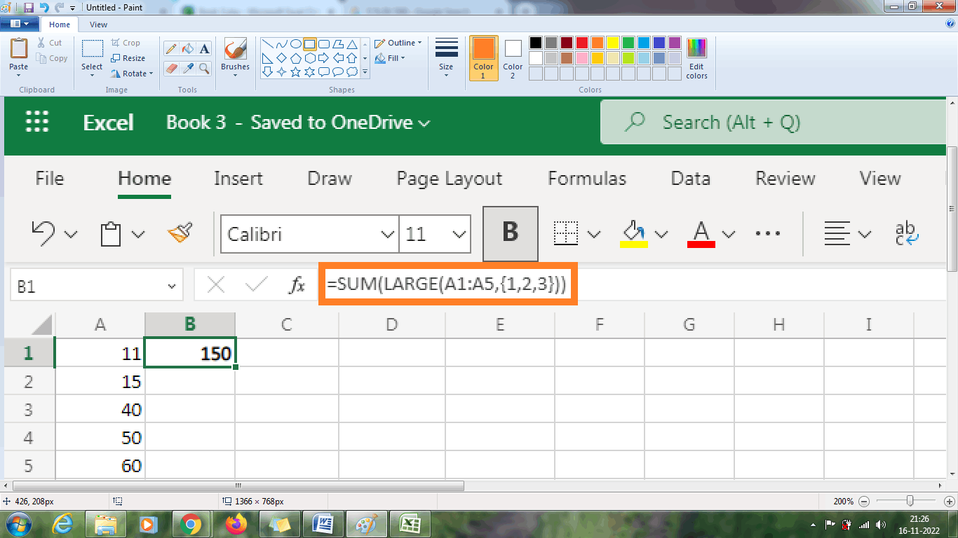
Example 4: Using the Array formula, how to sum the 'N' largest numbers?
To sum the ‘N’ largest number, the steps to be followed are,
1. Enter the data in a column from the range A1:A5.

2. Select a new cell to display the result of the sum of 'N' largest numbers. Enter the formula as =SUM (LARGE (A1:A5, {1, 2, 3}). Here the LARGE function is used to sum the 'n' largest numbers.
3. Press CTRL+SHIFT+ENTER or press Enter key. The array formula returns the sum of the largest three numbers in the respective cell.
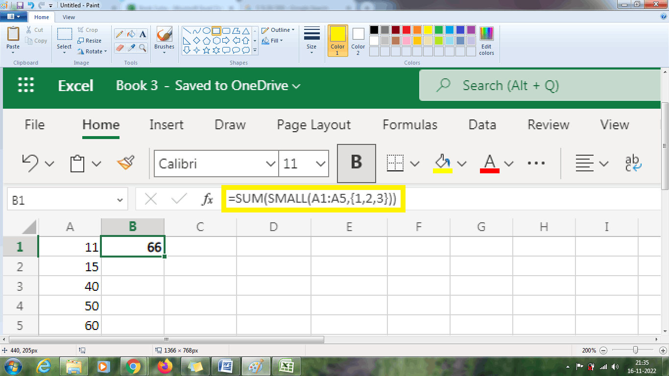
Example 5: Using the Array formula, how to sum the 'N' Smallest numbers?
To sum the ‘N’ smallest number, the steps to be followed are,
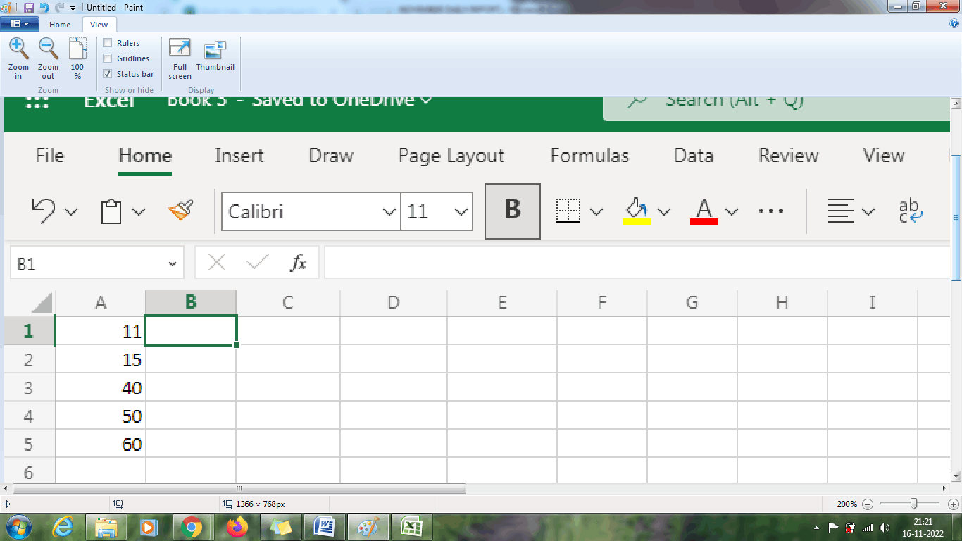
1. Enter the data in a column from the range A1:A5.
2. Select a new cell to display the result of the sum of 'N' smallest numbers. Enter the formula as =SUM (SMALL (A1:A5, {1, 2, 3}). Here the SMALL function is used to sum the 'n' smallest numbers.
3. Press CTRL+SHIFT+ENTER or press Enter key. The array formula returns the sum of the three smallest numbers in the respective cell.
Example 5: Array function for applying multiple conditions
In this example, the array function calculates the data using multiple conditions. The steps to be followed are,
1. Enter the data in the spreadsheet in the respective row and columns.
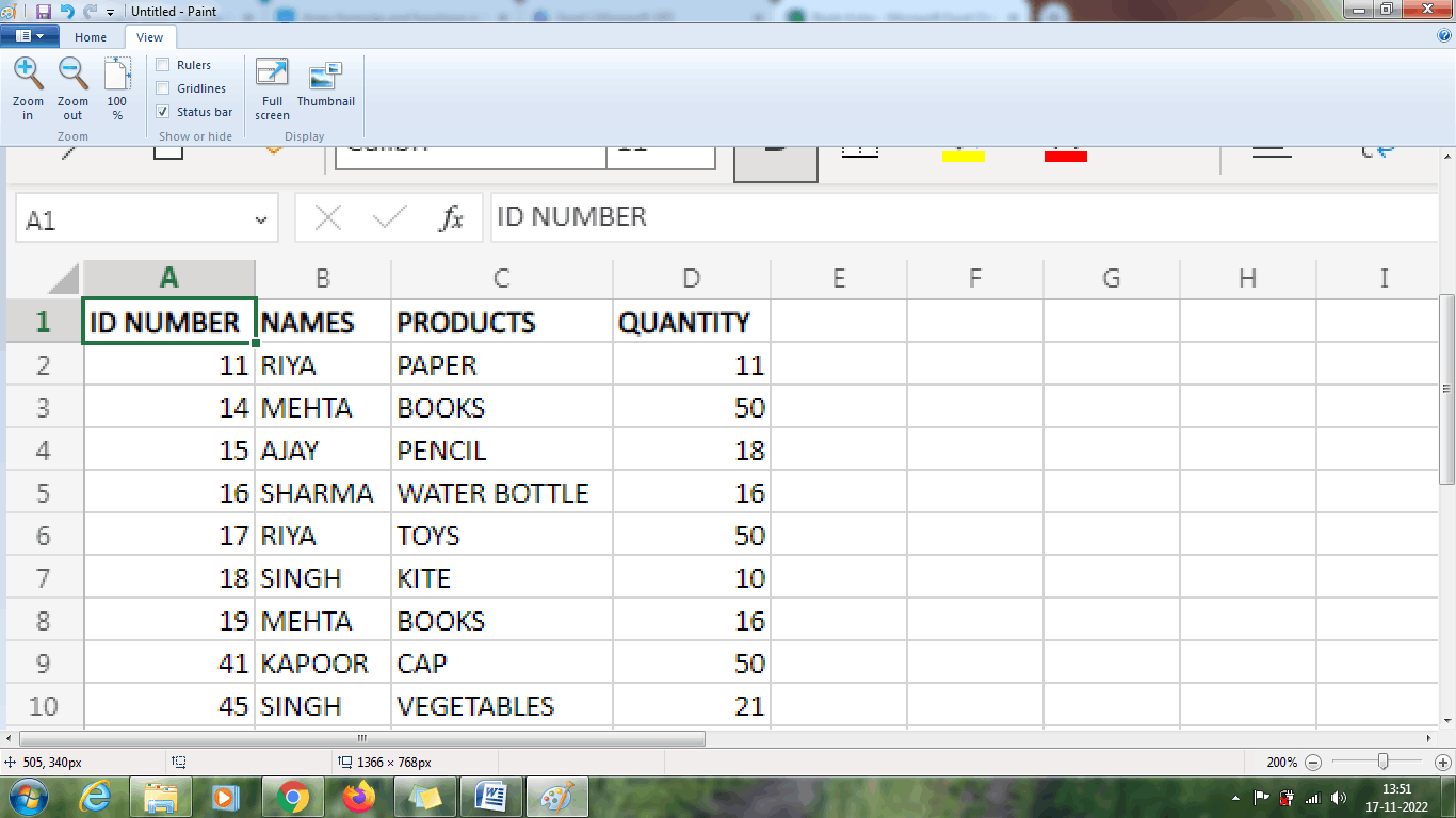
Step 2: To find the order taken by Mehta, the formula to be used as =SUM (COUNTIFS (B2:B10, "Mehta", C2:C10 {"Books"})) is entered in the new cell. Here COUNTIFS function is used to calculate multiple conditions, where the formula includes multiple conditions.
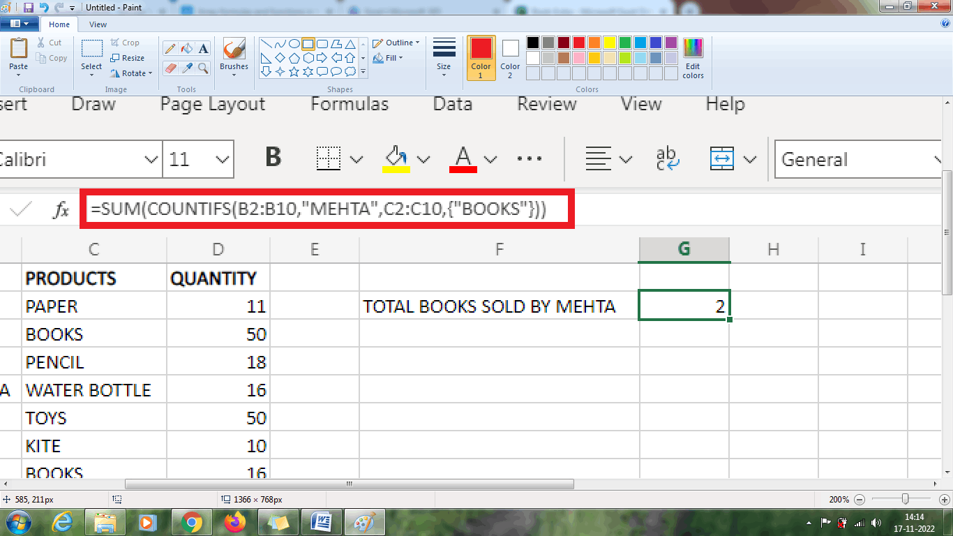
From the above worksheet, the result is displayed as 2, which Mr. Mehta sells the number of orders (BOOKS)
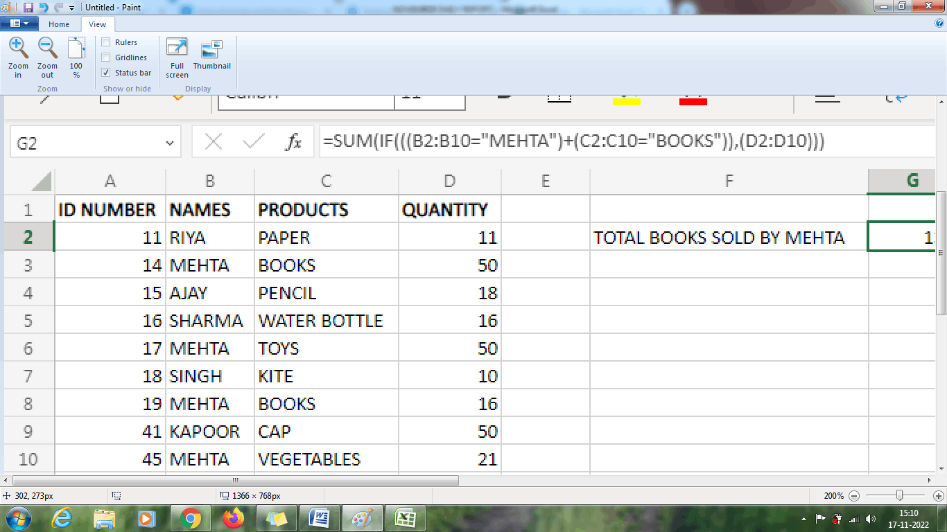
Example 6: OR operator in Array
Using OR operator in Excel, it displays TRUE if any of the conditions are applicable. The steps to be followed to use OR operator is,
1. Enter the data in the spreadsheet in the respective row and columns.
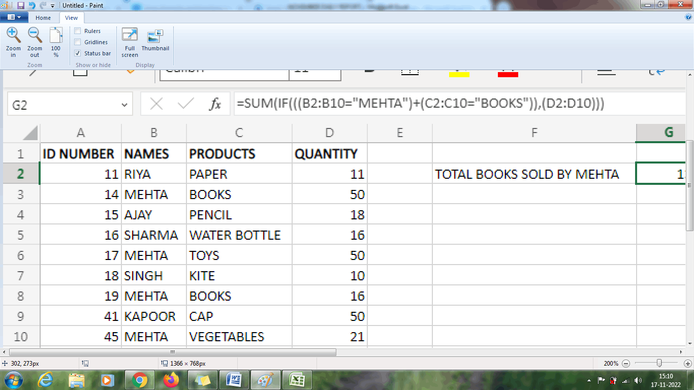
2. To count the Number of Books Sold by Mehta, enter the formula in the cell using OR operator as =SUM (IF (((B2:B10=”MEHTA”) + (C2:C10=”BOOKS”)), (D2:D10)))
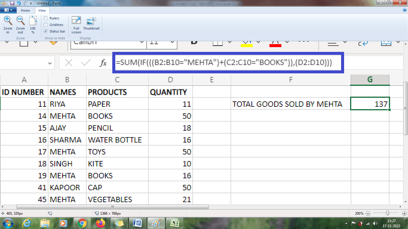
From the above worksheet, the result is displayed as 137, which is the total goods sold by Mehta. The OR sums the goods, including (BOOKS, TOYS, and VEGETABLES) as the function includes the data if anyone of the condition is true.
Example 7: AND operator in Array
The AND operator in Excel displays TRUE if all the conditions are applicable. The steps to be followed to use AND operator are as follows,
1. Enter the data in the spreadsheet in the respective row and columns.
2. To count the Number of Books Sold by Mehta, enter the formula in the cell using AND operator as
=SUM ((B2:B10=”MEHTA”) *(C2:C10=”BOOKS”)*(D2:D10))
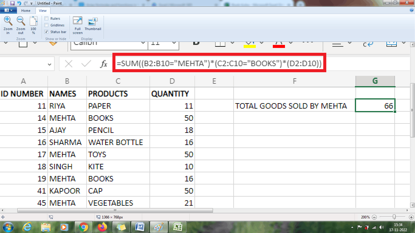
From the above worksheet, the result is displayed as 66, which is the total number of books sold by Mehta. The AND function returns the result if all the conditions are true, which means it sums only the goods of Books.
Unary operator in Array
Excel provides a default unary operator symbol called (--), called a double dash. The purpose of the double dash unary operator is to convert the non-numeric values into 1 or 0, where the array function can understand. The methods to use the unary operator in Array are as follows,
1. Enter the data in the respective column, namely A1:A5. Here the various dates are entered in the column.
2. Select a new cell, B1, to type a new value to find how many times a particular month's dates are repeated.
3. Select a new cell and enter the formula as
=SUM (--(MONTH (A1:A5) =B1)). Here B1 contains the value of '7', where the formula finds how many times the month 'JULY' is repeated.
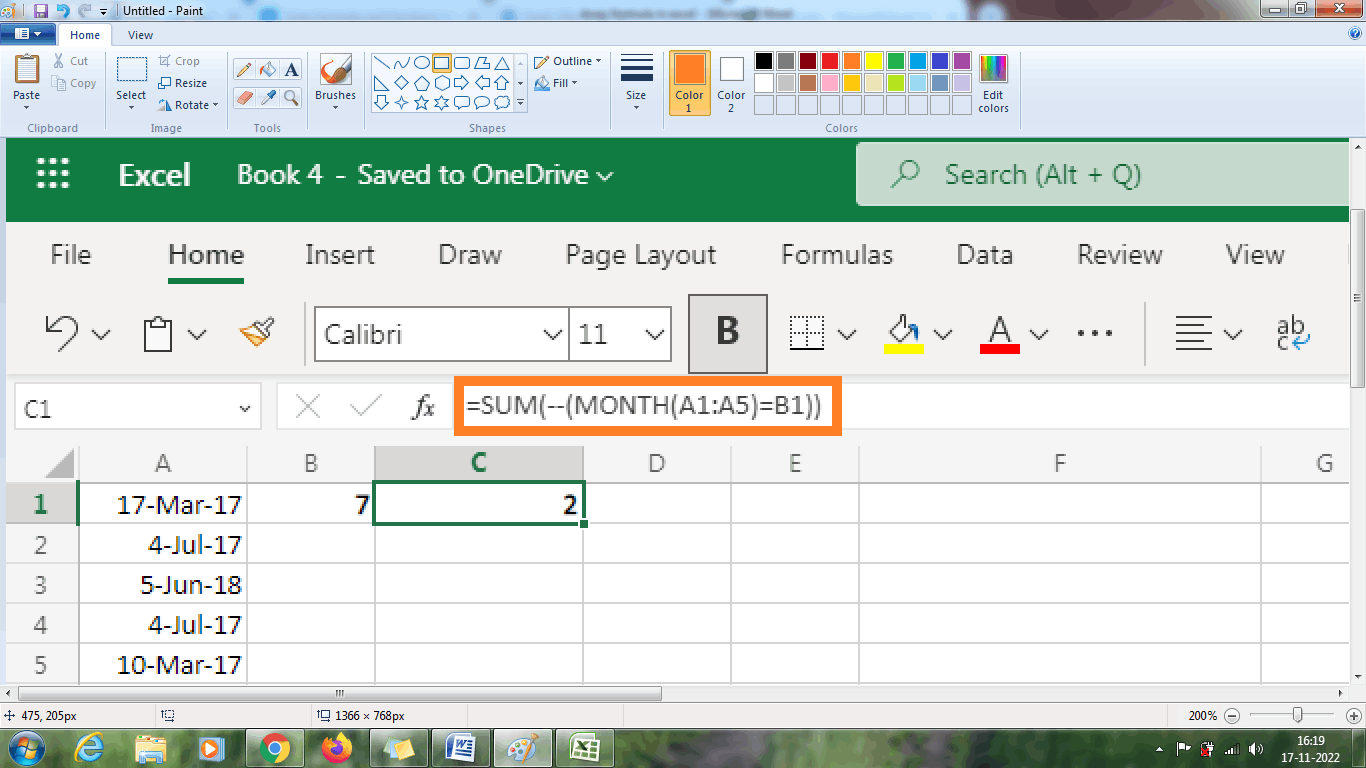
From the above worksheet, the value is displayed as 2 where the column ranges A1:A5 contains two July month data. Here the Array takes 1 as 'January', '2' as February,' 3' as March so on so. Similarly, '7' indicates the July month which needs to be counted.
Summary
From the above method, the various functions and methods of the Array formula are explained clearly.