Paste Options in Excel

Excel spreadsheet is a combination of numeric values, alphabets which is used for calculation purposes. While performing the calculations, there is a need to repeat the data for further process. To repeat the data, copy and paste the options is necessary. Excel provides various default options to copy and paste the data. The copy and paste options copy the data includes formulas, formats, comments and validation. Using Copy and Paste options or pressing Ctrl+C and Ctrl+V all the attributes is copied. To paste only the selective data or specific values use Paste option or select an option from the Paste Special option.

Different types of Paste Options

The different types of Paste Options in Excel are,

Paste Menu Option

The steps to be followed to use the paste menu option are,

Step 1: Enter the data in the respective cell namely A1:B5.

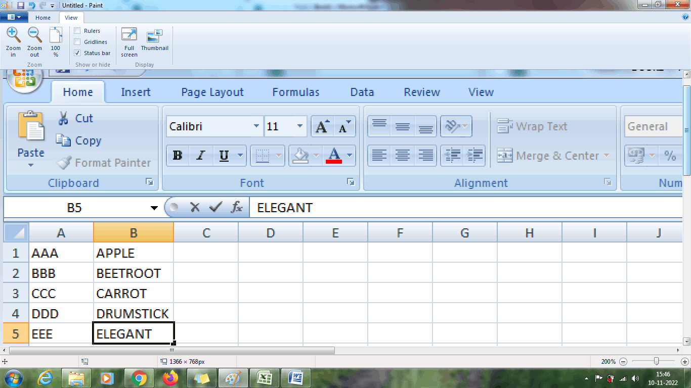
Step 2: Select the cell which contains the data that needs to be copied.

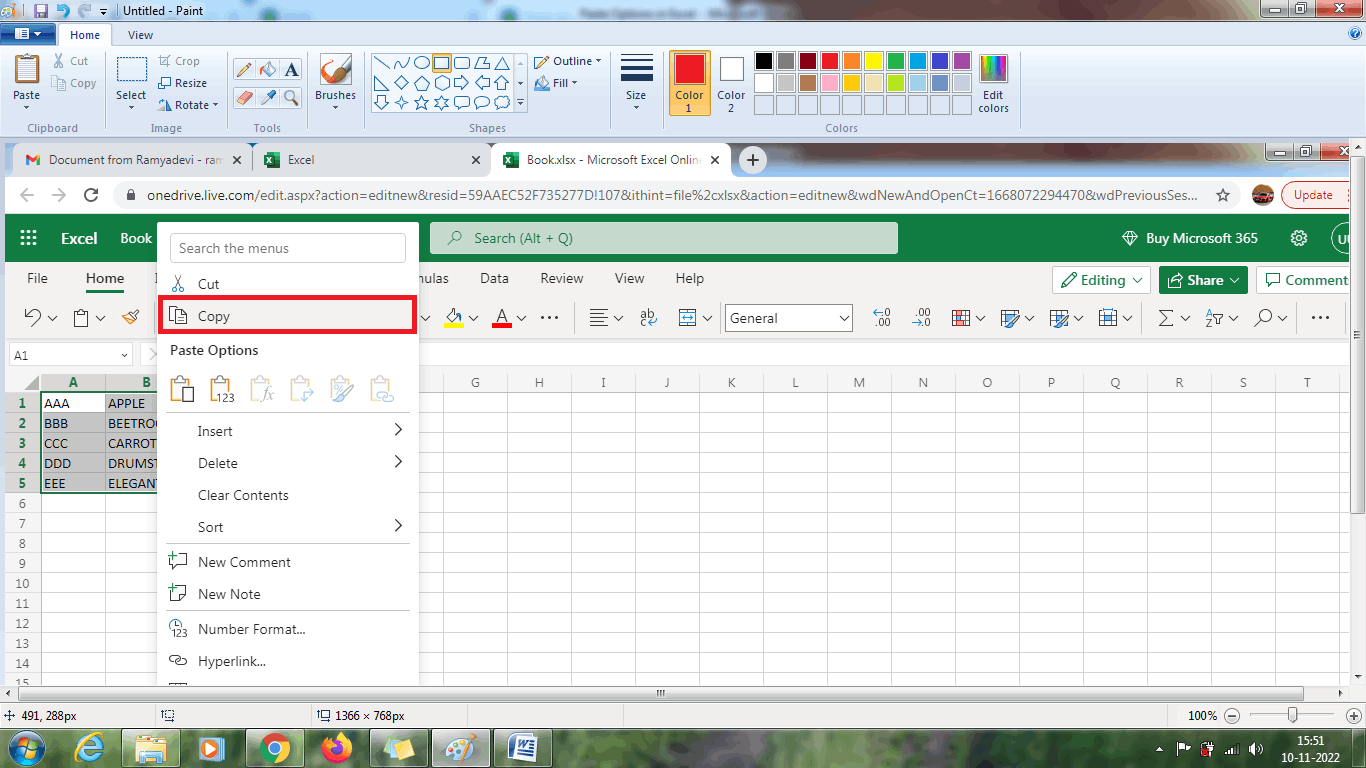
Step 3: Right click the data, choose the copy option from the menu or press Ctrl+C.

Step 4: Select the range of new cells D1:E5 namely where the data needs to be copied.

Step 5: Choose the Paste option from the Home Tab, where there displays multiple paste option under the Paste menu.

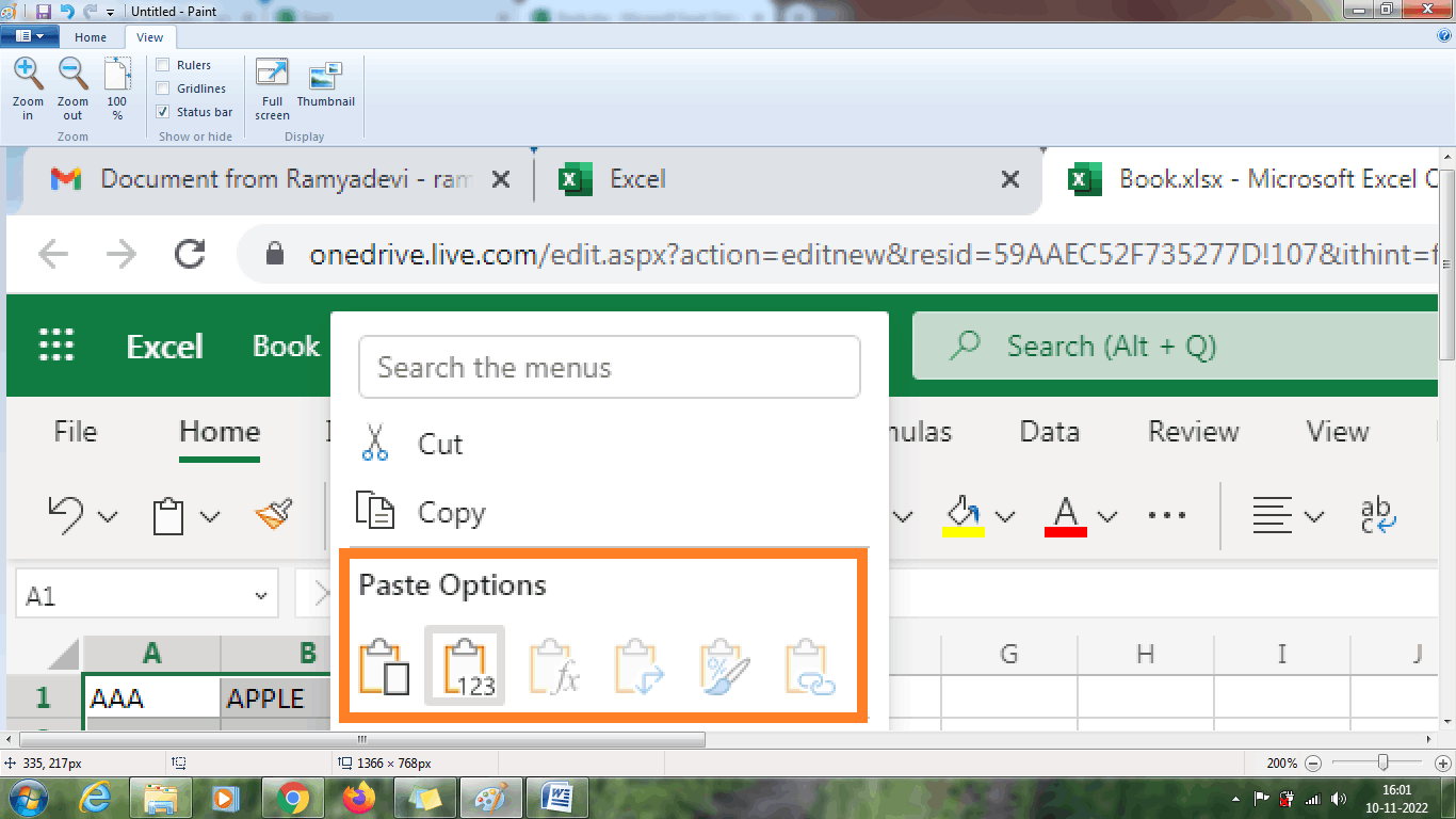
The paste option is subdivided into following types,

Paste- It pastes all the contents or data, formatting present in the cell including linked data.

Values- The value option is used to paste the result of the formula.

Formulas- The formula option is used to paste only the formula.

Formatting- The formatting option only pastes the formatting.

Paste Special- The paste special option is to paste the selective data from the given data.

From the above menu, the paste option is selected.

Step 6: Click on the Paste Menu, the data is pasted in the selected location.

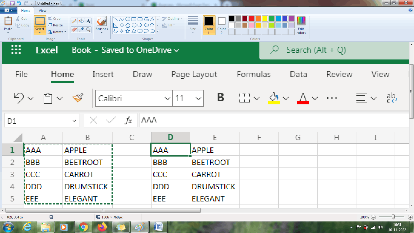
From the above worksheet, the data is pasted in the selected cell range namely D1:E5.

How to use Value function to copy and paste the result?

As described earlier, a method called value, which is used to copy and paste the result.

The steps to be followed to use the value function are,

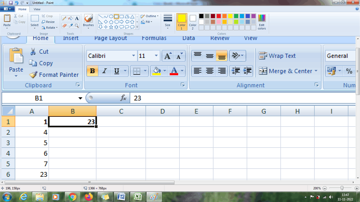
Step 1: Enter the data in the respective cell namely A1:A5. Here the result is added from (A1+A2+A3+A4+A5) and display in the cell A6.

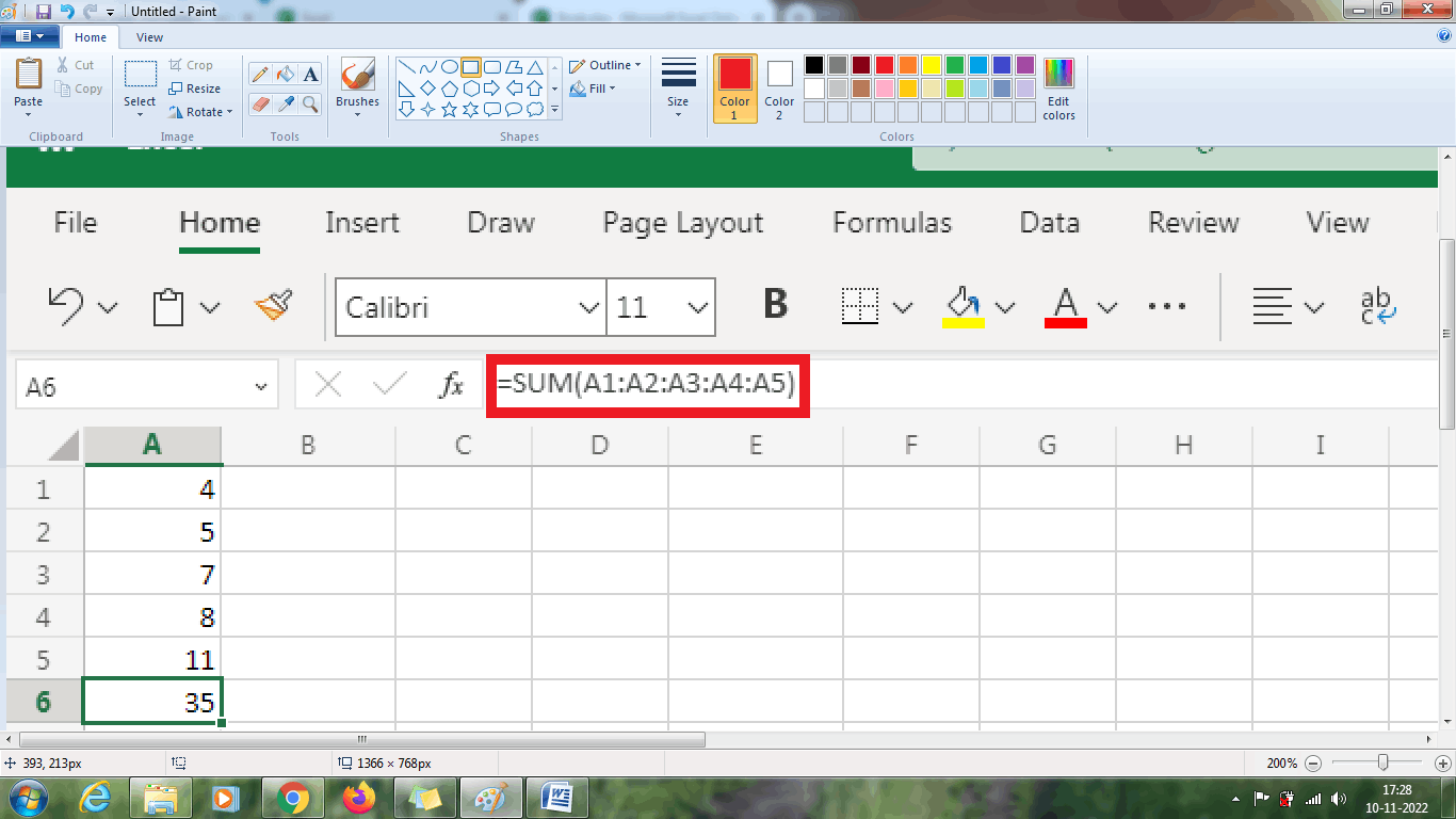
Step 2: Select the result present in A6.

Step 3: Right click the data, choose the copy option from the menu

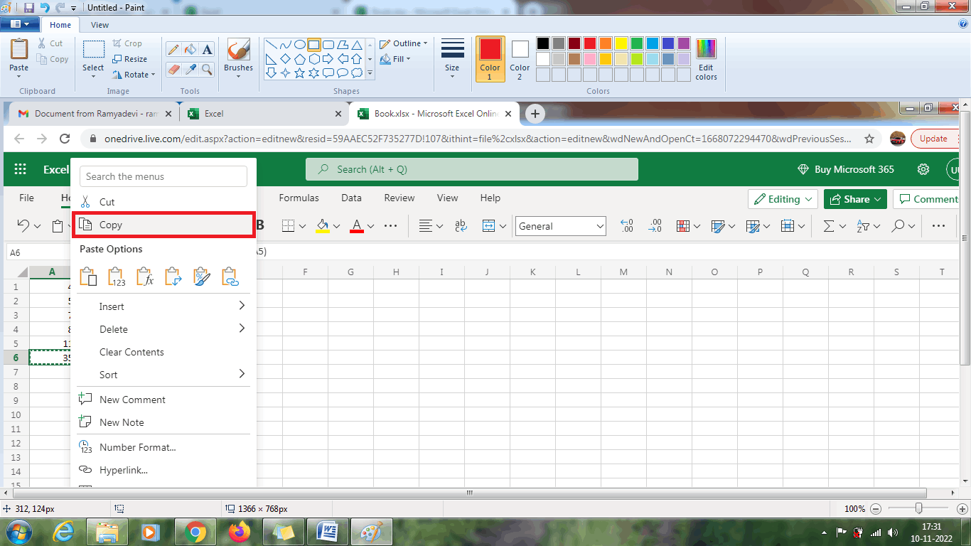
Step 4: Select a new cell where the result wants to display namely C1.

Step 5: Click on the new cell and click right.  A menu will appear in that choose the value option.

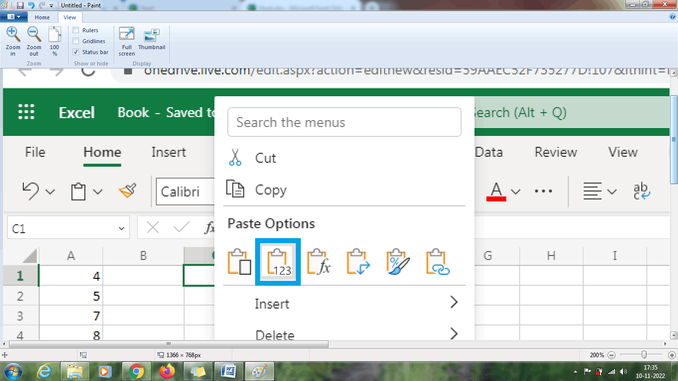
The blue colour indicates the value option.

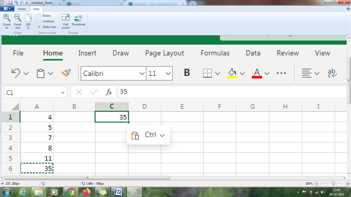
From the above worksheet, only the result is copied to the new location C1.

How to copy and paste specific content in Excel?

To copy and paste specific content or selective text in Excel, Paste Special option performs the task. If the required option is not present in the Excel, the Paste Special option is used. The steps to be followed to use Paste Special option are,

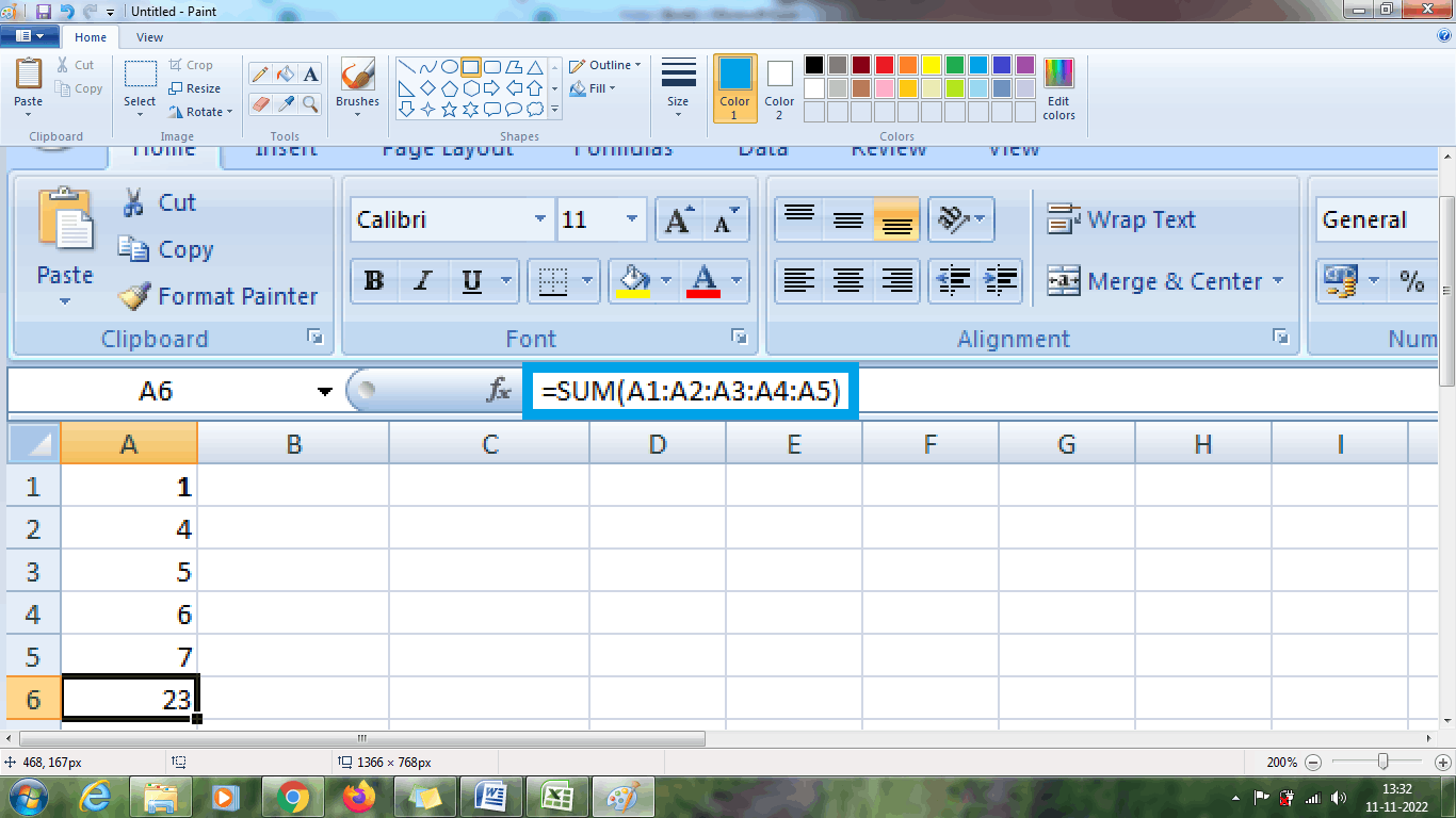
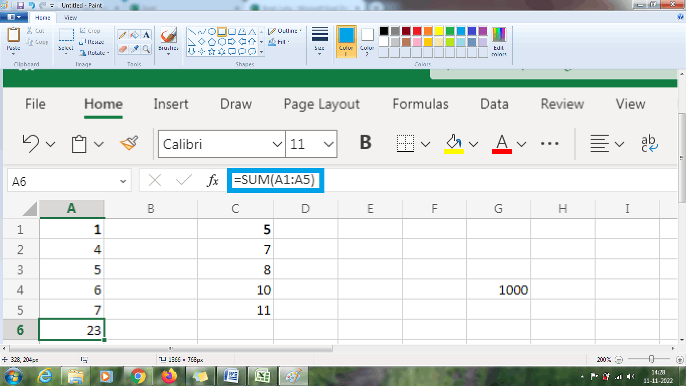
Step 1: Enter the data in the respective row range namely A1:A5, where the value needs to be added (A1+A2+A3+A4+A5)

Step 2: Select the cell A6, type the formula as =SUM (A1:A5). The result will display in the cell A6.

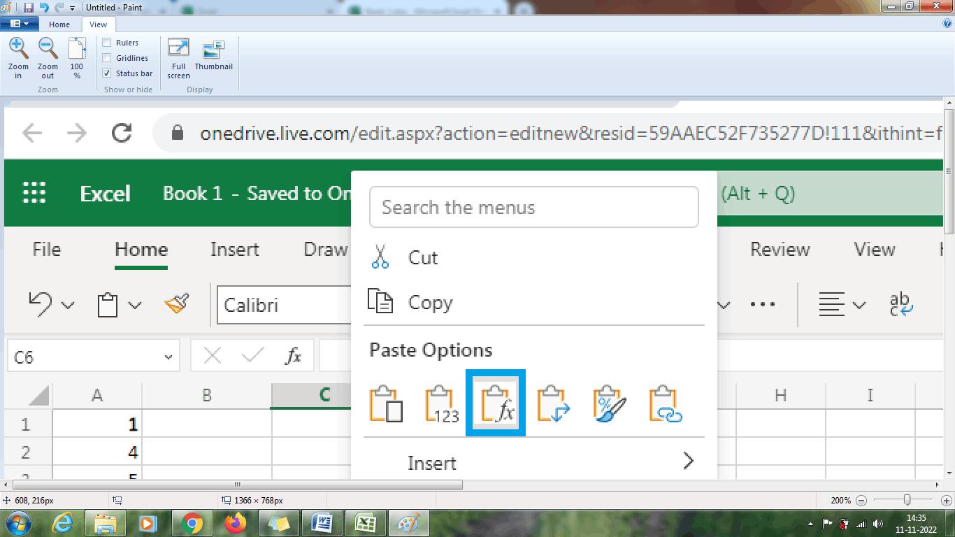
Step 3: Select the cell A6, press Ctrl+C or choose copy option from the Home tab

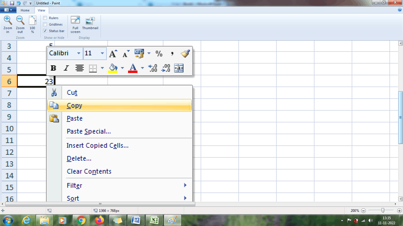
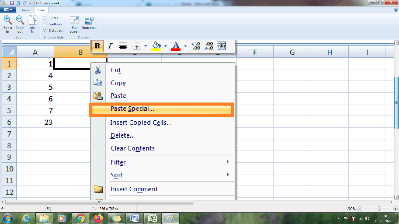
Step 4: Select a new cell namely B1, where the user wants the data to be pasted.

Step 5: Select the paste special option from the Paste option in the Home Tab.

Step 6: The Paste Special dialog box displays various options. In that choose the option. Choose the All option from the Paste option and “Add” from the operation menu. Click Ok.

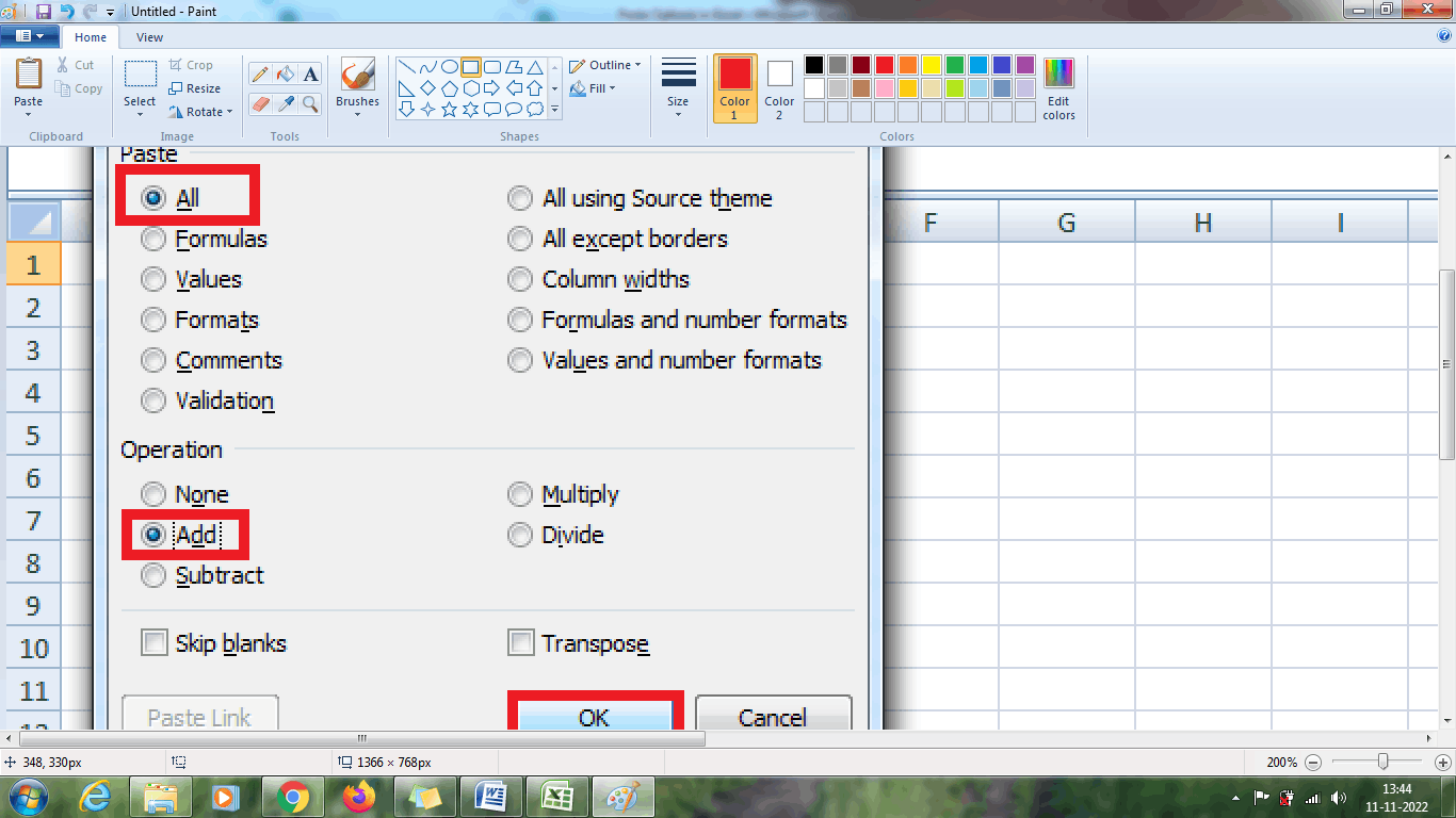
Step 7: The result of adding A1:A5 is pasted in the cell B1.

From the above worksheet, only the selective or required data is pasted in the cell B1.

How to use Formula function to copy and paste the result?

In large data set, the formula needs to be repeated for calculation purposes. Sometimes the user may forget the password and typing manually takes times, and error occurs rarely. To simplify this, Excel provides the default formula function to copy and paste the required formula for further calculation. The steps to be followed, to use the formula function are as follows,

Step 1: Enter the two sets of data in the respective row and column namely A1:A5 and C1:C5 to perform addition.

Step 2: In the cell A6, enter the formula as =SUM (A1:A5). The result will be displayed in the cell A6.

Step 3: Select the cell A6, press Ctrl+C or click the copy option from the Home tab.

Step 4: Select the cell C6, right click and select the Formula option from the Paste Menu

Step 5: The same addition formula is applied to the cell range C1:C5. The result is displayed as 41, which is the addition of cell range C1:C5.

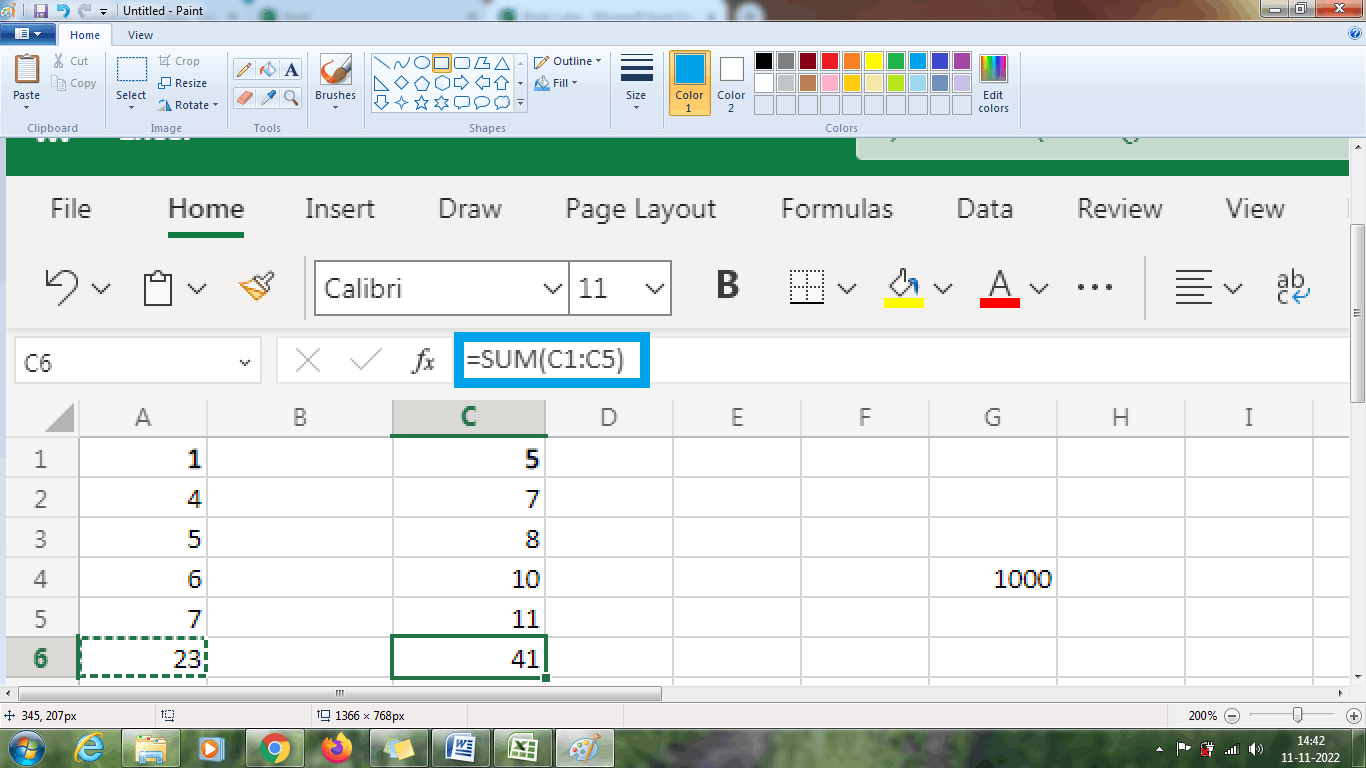
The result is displayed by copying and pasting the formula option.

How to use Transpose function to copy and paste the result?

Transpose is a method which is used to transfer the data set from vertical to horizontal range. This transpose function is used to sort the data in the formatted form. The syntax for Transpose is,

=TRANSPOSE (array)

The transpose is used in either formula method or in using default Transpose function present in Excel. The steps to be followed for implementing Transpose function are,

Step 1: Enter the two sets of data in the respective row and column namely A1:A5 and C1:C5.

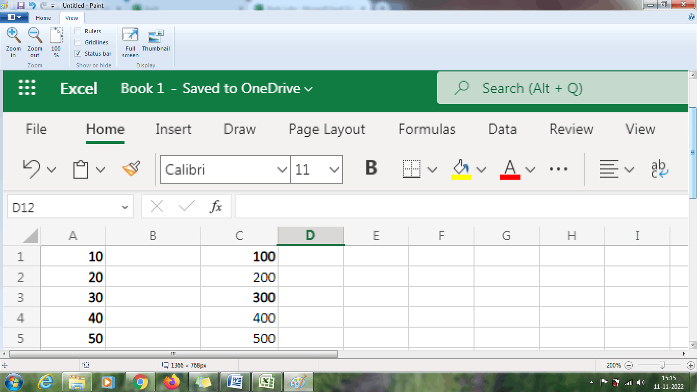
Step 2: Copy the data from A1:A5 and C1:C5 by pressing Ctrl+C or choose the copy option from Home Tab.

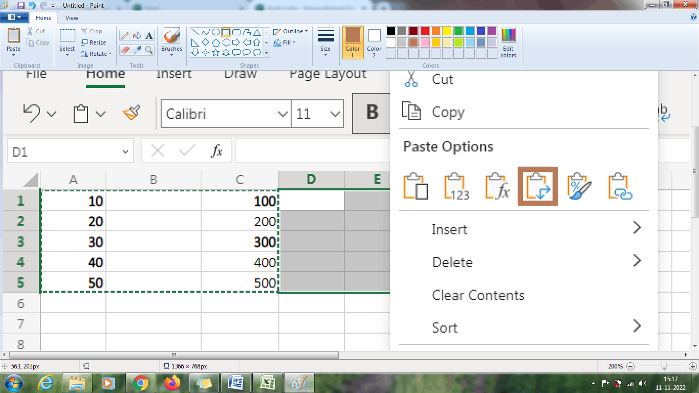
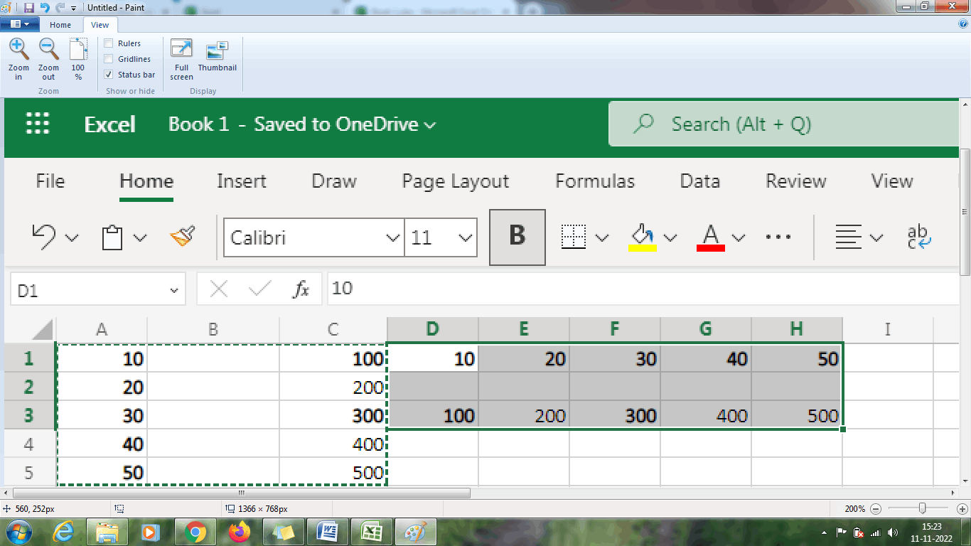
Step 3: Select the new cell range, where the user the user wants to display the selected data namely D1:H3. Here the cell range is selected as D1:H3, because the transpose function displays the data in vertical manner.

Step 4: Choose the transpose option from the Paste option. It displays the horizontal data in vertical range.

Step 5: The result will be displayed in the cell range D1:H3 in the vertical range.

How to use formatting function to copy and paste the result?

In Excel calculation, there is a need to copy and paste the data sometimes. It includes numeric values, alphabets etc. While copying the data, there is a requirement to paste the data along with background color, border, style etc. To copy the data along with formatting option, Excel provides default Format option to paste the data along with formatting changes. The steps to be followed to use the formatting option are,

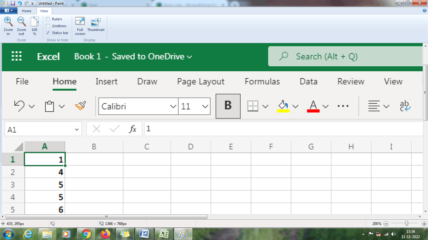
Step 1: Enter the data in the respective row namely A1:A5.

Step 2: Choose the required formatting option for the data.

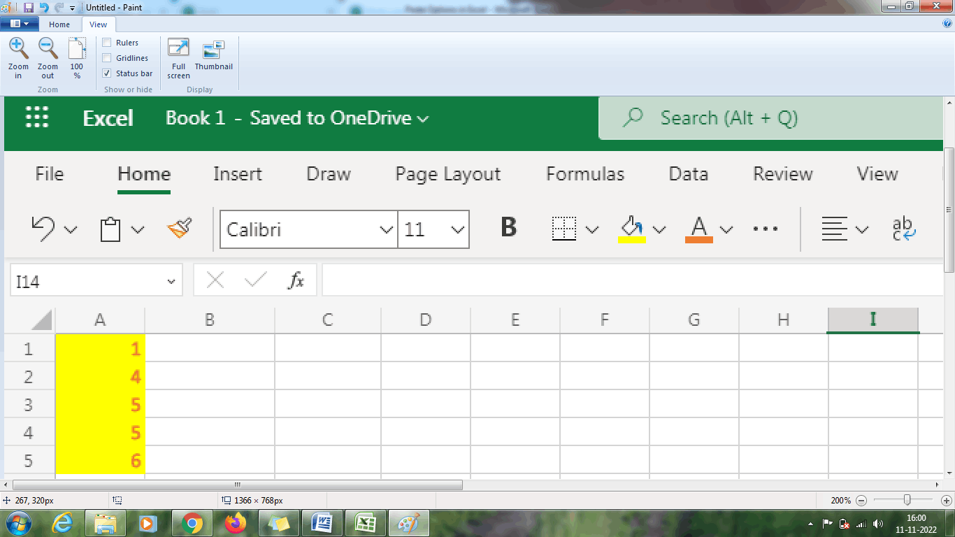
Step 3: Select the cell range A1:A5 and press Ctrl+C or choose the copy option from the Home Tab.

Step 4: Select the new cell range B1:B5, where the user needs to paste the formatting option.

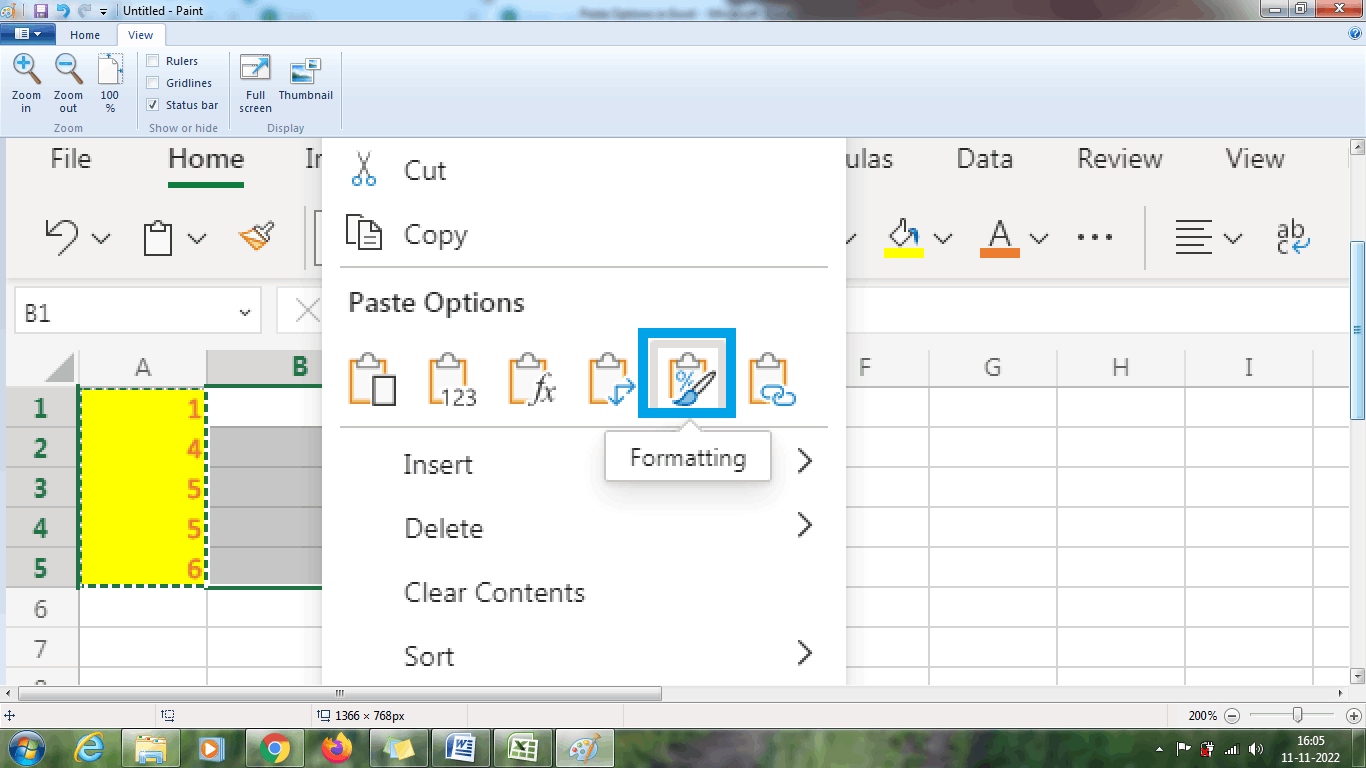
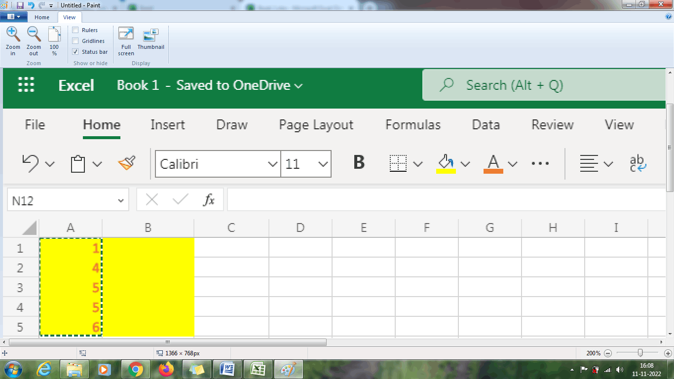
Step 5: The format option copies and pastes only the formatting changes. Hence the row B1:B5 is filled with formatting changes present in the cell range A1:A5.

How to use the Link function to copy and paste the link in Excel?

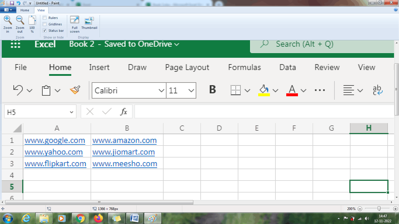
Excel worksheet contains numeric values, alphabets, website links etc. To copy and paste the links the steps to be followed are.

Step 1: Enter the required link in the respective row or column namely A1:B3.

Step 2: Select the cell range A1: B3 and press Ctrl+C or choose the copy option from the Home Tab.

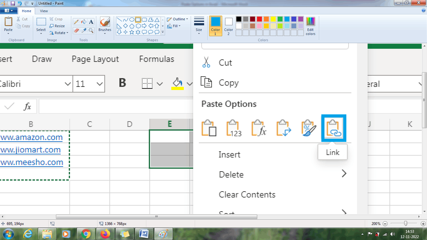
Step 3: Select the new cell range namely E1:F3 where the user wants to display the result.

Step 4: Choose the link option from the paste menu. Therefore the link is pasted to the selected location.

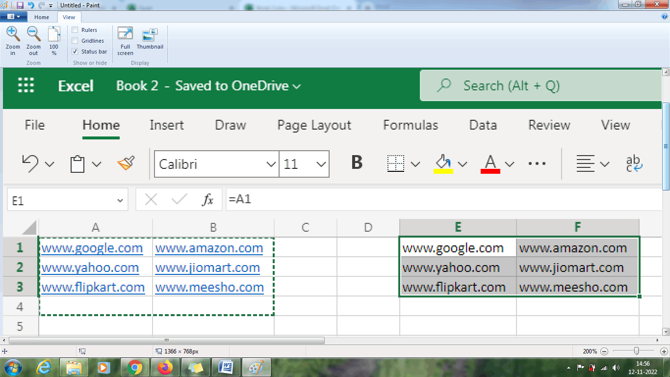
Step 5: The link is pasted to the new location using the link function.

Summary

From the above tutorial, the various methods and functions to copy and paste the data is explained briefly.