Reverse List in Excel

What is Reverse list in Excel?

Microsoft Excel is widely used for calculation purposes like statistical and analytical for predicting and getting the result. Sometimes for calculation purposes, the user needs to shuffle the data or flip the order of the data upside down in a vertical dataset and left to right in a horizontal dataset, which means reversing the data or list. Doing manually take lot of time, and sometimes leads to error. Excel provides default function to reverse the list of data present in the worksheet using formulas, simple sorting trick or VBA. It provides default functions like INDEX, COUNTA, SORTBY, SEQUENCE and ROW functions for reversing the data present in the list. It provides several methods to use the reverse function with and without formulas. In this tutorial the various methods for reversing the list is explained clearly.

1. Reversing the list without using the formula

In the following method the data in the list are reversed without using the formula. If someone forgets the formula or function, easily this method can be applied for reversing the list or range.

1. Enter the list of values in the spreadsheet. Here the values are entered from cell range A1:A10.
2. From the cell B1:B10 enter the numeric value from 1 to 10 .Like ‘1’ in cell B1, ‘2’ in cell B2. Similarly follow this step up to value 10
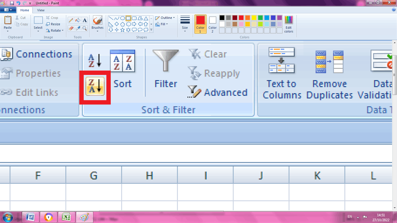
3. Select any of the data in the column B1:B10. Choose Data> Sort Descending to Ascending order in the ribbon tab in Excel
4. The data in the column A2:A11 will change its order, and the values present in the column B2:B11 will also changes.

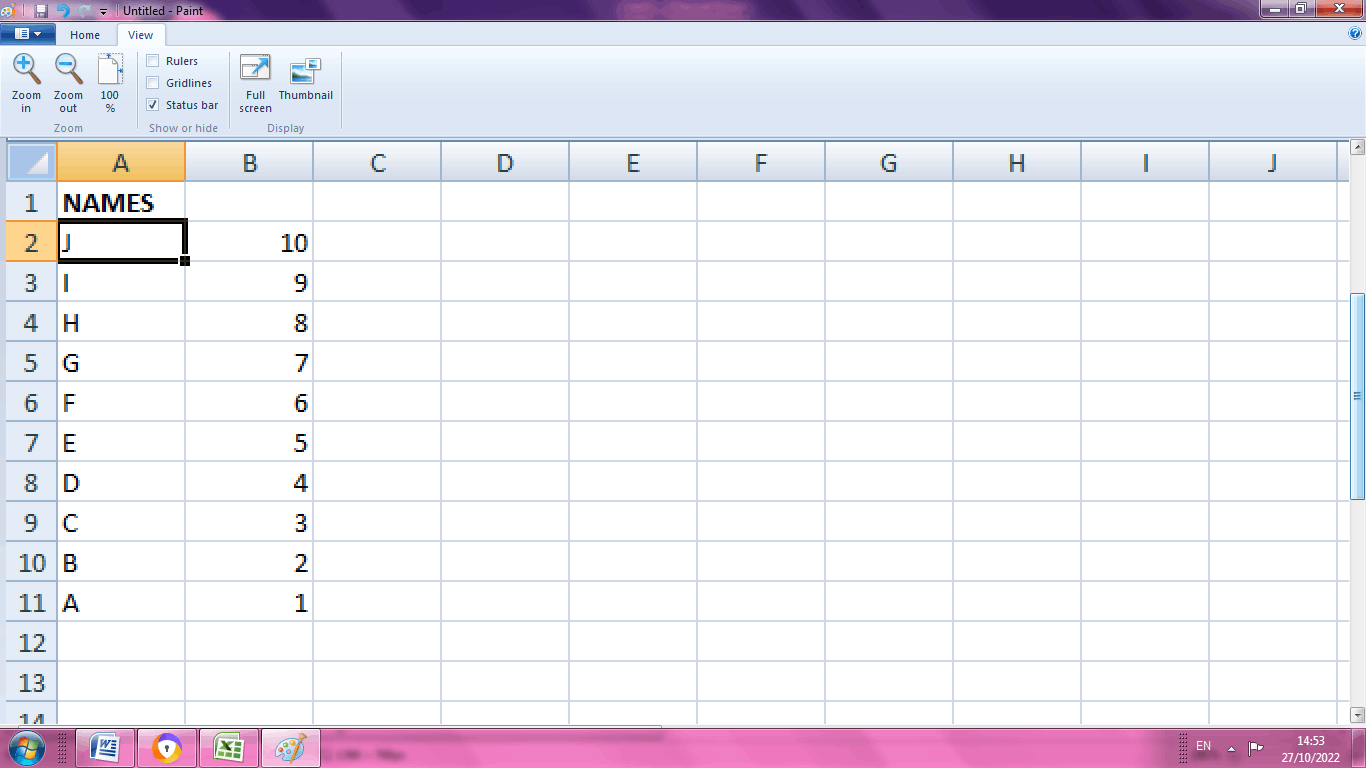
From the above worksheet, the data are reversed, where the value ‘A’ present in the bottom of the list while ‘J’ present in the top of the list. The numbers present in the column B2:B11 is called helper column, where it is used to reverse the order of the list.

2. Reversing the list using the formula

One can reverse the list using the Excel default formula. Here the combination of INDEX and ROWS function is used to reverse the list or range in Excel. To use this formula, following steps are followed.

1. Enter the data in the worksheet in the required column.
2. Select a new cell where the result wants to display and enter the formula as =INDEX (CELL RANGE, ROWS (CELL RANGE). Here the formula used are = INDEX ($A$2:$A$11, ROWS (A2:$A$11).
3. It display the result in the cell B2. Drag the formula towards the cell B11. It will display the result in remaining cell. This process is called spilling. The process of spilling is done in Excel 365 and some advanced versions like Excel 2021.

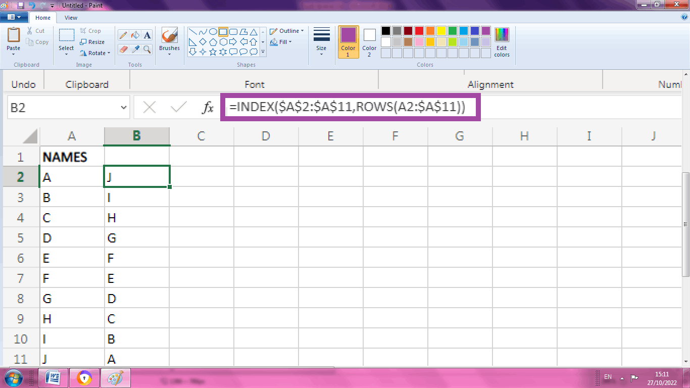
From the above worksheet, the data is reversed using the function INDEX and ROWS. Here the data range containing the list A2:A11 becomes the first argument of the array function. To return the last element of the array, ROW function is used.

3. How to reverse the order using SEQUENCE, SORTBY and ROWS function together?

The list or range in the cell can be reversed using the Excel default function called SEQUENCE, SORTBY and ROWS function. It is called as Dynamic array formula which is used for quicker and efficient calculations .To use this function following steps are followed,

1. Enter the data in the spreadsheet in the required column
2. Select a new to create the sequence for the column range A1:A10. Enter the formula as =SEQUENCE (10, 1, 1, 1). The arguments present in the Sequence function is ‘10’ represents the number of rows, ‘1’ represents columns, ‘1’ represents the start, ‘1’ represents the step. It displays the sequence of numbers in the column B1:B10.

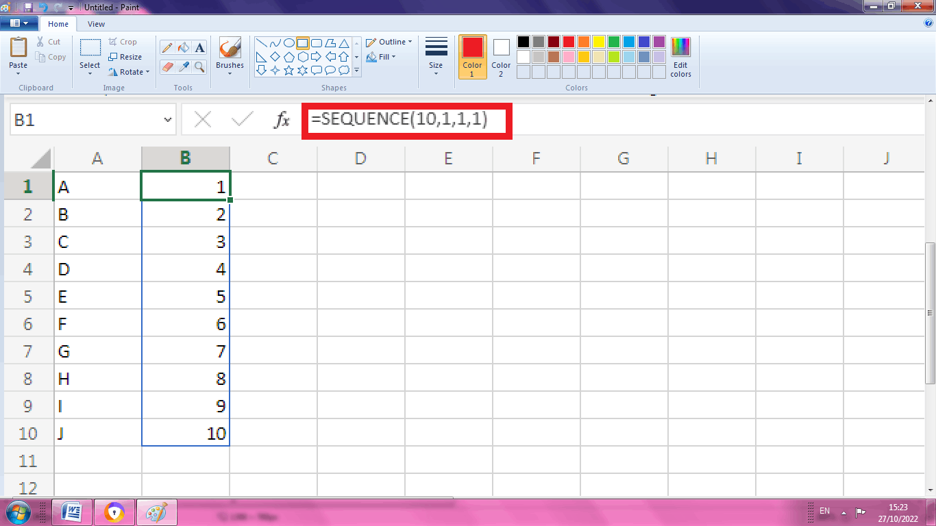
From the above worksheet, the sequence is created using the sequence function. The action of spilling is performed to fill the remaining cells.

• Next use SORTBY function, by selecting a new cell and enter the formula as =SORTBY (A1:A10, B1:B10,-1). Here -1 indicates the values to be arranged from descending to ascending order.

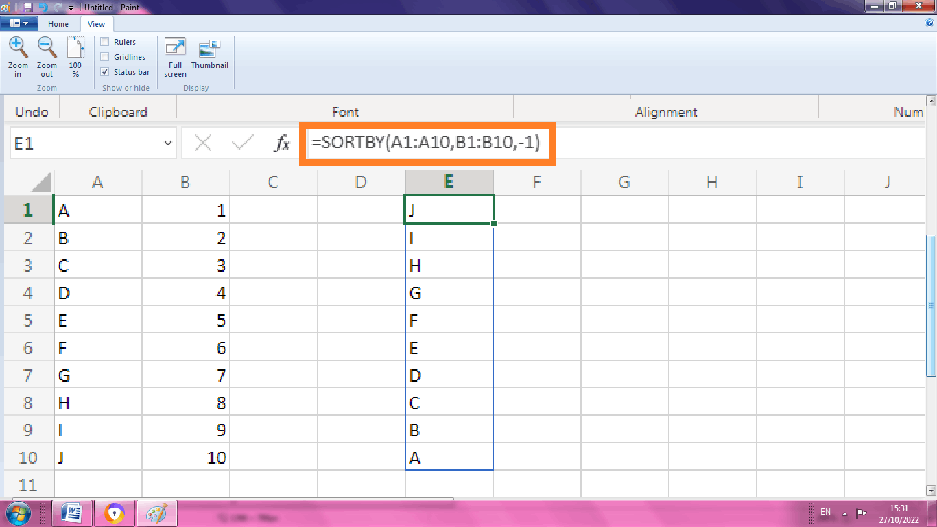
Here the values are reversed using SORTBY function.

• Next, use the SEQUENCE function inside the SORTBY function. Select a new cell and type the formula as = SORTBY (A1:A10, SEQUENCE (10, 1, 1, 1),-1). Here the arguments ‘10’ represents the rows, 1- column, 1- start, 1- step and -1 indicates the range to be arranged from descending to ascending order.
• Next step involve the merging of ROWS function inside the formula. Select a new cell and type the formula as = SORTBY (A1:10, SEQUENCE (ROWS (A1:A10), 1, 1, 1),-1). The ROW function is used to count the number of rows in a range.

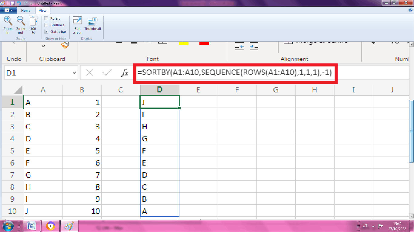
From the above worksheet, the SEQUENCE, SORTBY and ROWS function is used together to reverse the list or range in the table.

4. How to reverse the list of range using COUNTA function?

Excel default function called COUNTA is used to reverse the list or range in the table. The formula to be used is,

=INDEX (list, COUNTA (list) +ROW (list)-ROW (), 1).

To implement this formula, steps to be followed are,

1. Enter the data in the worksheet in the required column.
2. Select a new cell and type the formula as =INDEX (A1:A10, COUNTA (A1:A10) +ROW (A1:A10)-ROW (), 1). Here A1:A10 is considered as list.
3. The result will be displayed in the cell.

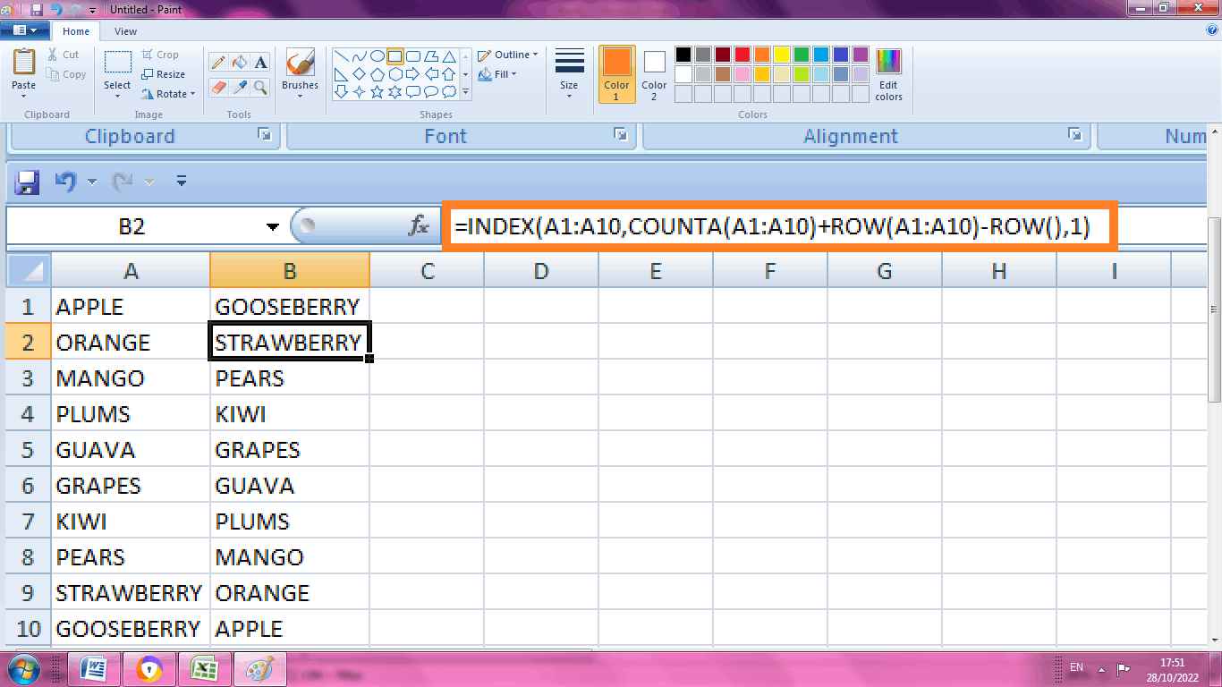
From the above worksheet, the list is reversed using the formula INDEX, COUNTA and ROW. The name “list” is a named range, where it is an absolute reference by default. In this formula INDEX function acts as a important part of the formula, where it represents the list as an array of argument. The other part of the formula is called expression, which represents the correct row number in the formula.

COUNTA- It is used to represent the count of non-blank cell present in the list. In this example ‘10’ is represented as non-blank cell

ROW – It is used to represent the starting row number. For example, the row number here is 1.

ROW () - It represents the row number where the formula is present.

5. How to reverse the list horizontally?

Excel default functions or formula is used to reverse the column in a vertical manner. Similarly using this function, the data in the row can be flipped or reversed in a horizontal manner. To reverse the data horizontally, following steps are followed,

1. Enter the data in the respective row. Here the data are entered in the row range namely A1:J1
2. Enter the helper column number 1 to 10 in the row A2:A10.
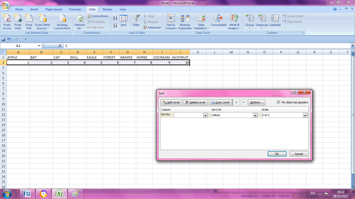
3. Select the value and helper column range ,here in the example the data range to be selected are A1:J2.
4. Choose the Sort icon from the Data Tab. A dialog box will appear, in that select the option button. The sort option dialog box will appear, in that choose “Sort left to Right” option. Click OK.

From the above dialog box, click the “OPTION” button.

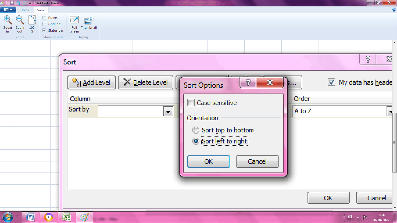
• Click OK, after choosing the “Sort Left to Right button”.

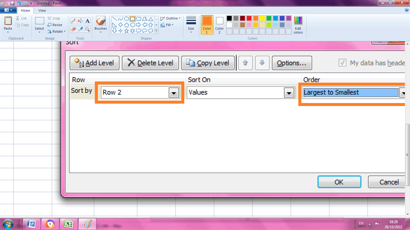
• From the above worksheet, choose the helper row in Sort by option. Here the helper row is present in row 2. Hence row 2 is selected. In order choose the “Largest to Smallest option”. Click Ok.

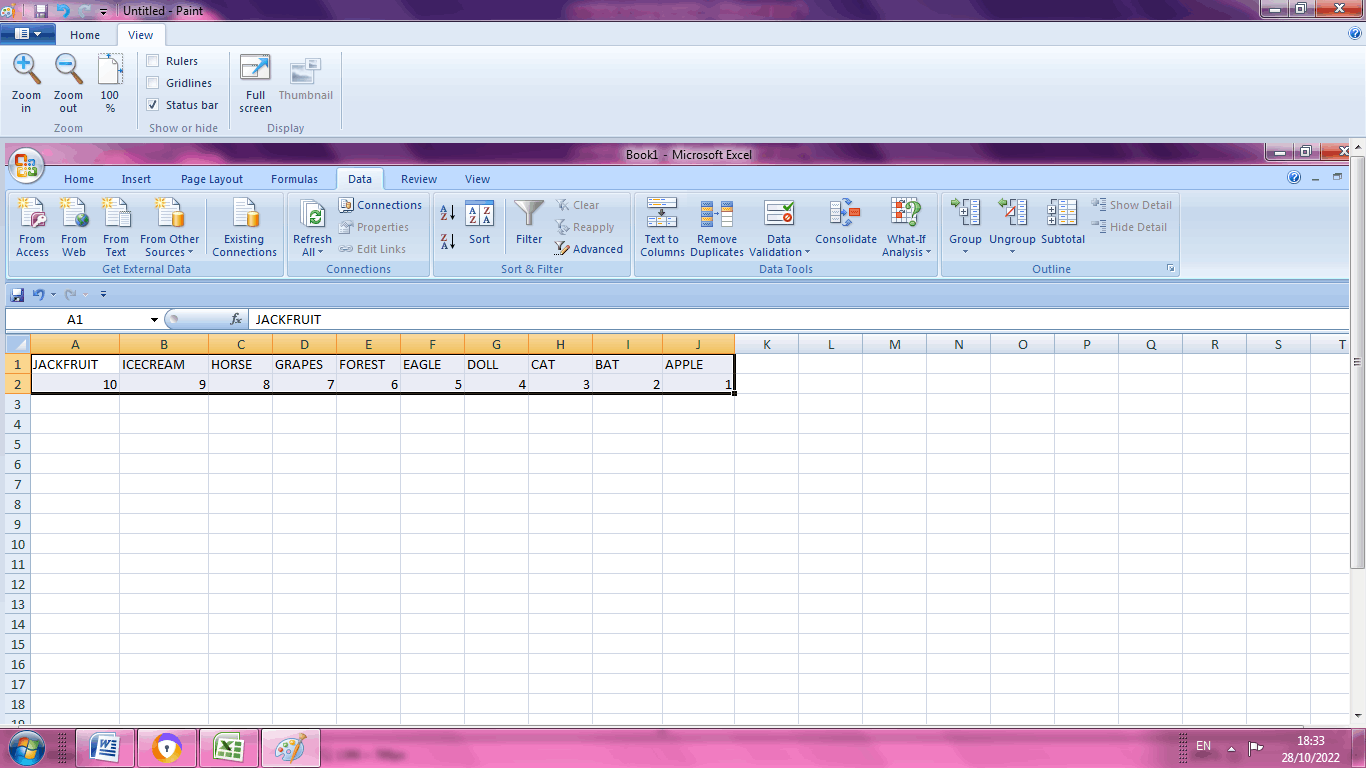
From the above worksheet, the data are reversed in the order.

Summary

From the tutorial, the various methods and functions to reverse the order is explained briefly.