Locate Maximum Values in Excel
Excel is a combination of numeric values and numbers. To retrieve the result, Excel provides various formulas and functions. Sometimes the user needs to find the largest value from the given data. Searching manually takes more time and is difficult for a large set of data. To locate the maximum values easily, Excel provides a function called MAX to find the values easily.
MAX Function
The MAX function in Excel represents the maximum value from the given data sets.
Syntax
MAX (number 1, [number 2] .....)
The syntax's arguments can be numeric values, alphabets, arrays, or any references.
Example 1: The steps to use the MAX function are as follows,
Step 1: Enter the range of data in column A1:A10.
Step 2: Select a new cell where the user wants to display the result and type the formula as =MAX (CELL RANGE).
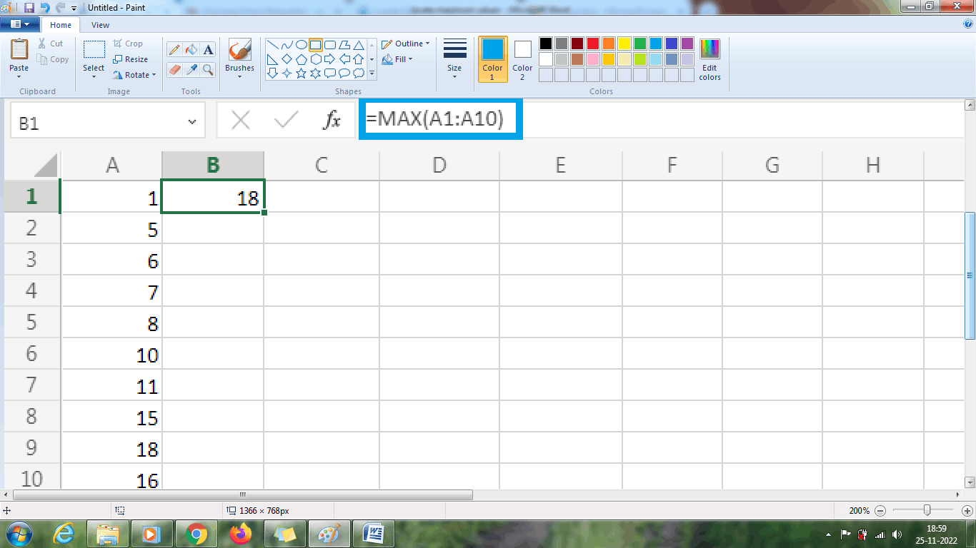
From the above worksheet, the result is displayed as 18, which is the maximum value in the column range A1:A11.
MATCH Function
The MATCH function searches for the required or selective item from the given data set and displays the data's position.
Syntax
MATCH (lookup _value, lookup_array, [match type])
lookup_value – Value which is matched with the looup_array
lookup_array – The range of cells which is searched.
Match_type – The match_type value indicates the Excel matching the lookup_value with lookup_array.
Example 2: How to display the row number of the maximum value in the given data?
The MATCH function is used along with the MAX value to display the row number of the maximum value. The steps to be followed are,
Step 1: Enter the range of data in column A1:A10.
Step 2: Select a new cell where the user wants to display the result and type the formula as =MATCH (MAX (A: A), A: A, 0)
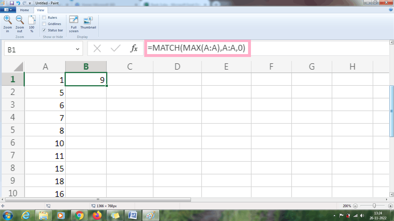
The MATCH function retrieves the data as (18, A: A, 0), 9. The above worksheet displays the result as nine, which is the row number of the data 18. As the number 18 is the largest value in the given data, the MATCH function displays the respective row number. Hence the MATCH function returns the position of the maximum value.
Example 2.1: How to display the row number of the specified data?
To display the row number of the specified data, the MATCH function is used. The steps to be followed are,
Step 1: Enter the range of data in column A1:A10.
Step 2: Select a new cell where the user wants to display the result and type the formula as =MATCH (50, A1:A10, 0)
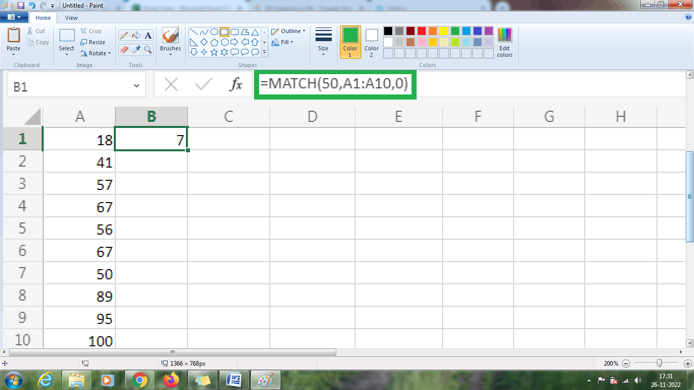
The above worksheet shows the result as 7, where the number 50 is present in row 7.
Example 2.2: What will result if the specified number is not present in the data?
To display the specified date, the MATCH function is used. The steps to be followed are,
Step 1: Enter the range of data in column A1:A10.
Step 2: Select a new cell where the user wants to display the result and type the formula as =MATCH (81, A1:A10, 1)
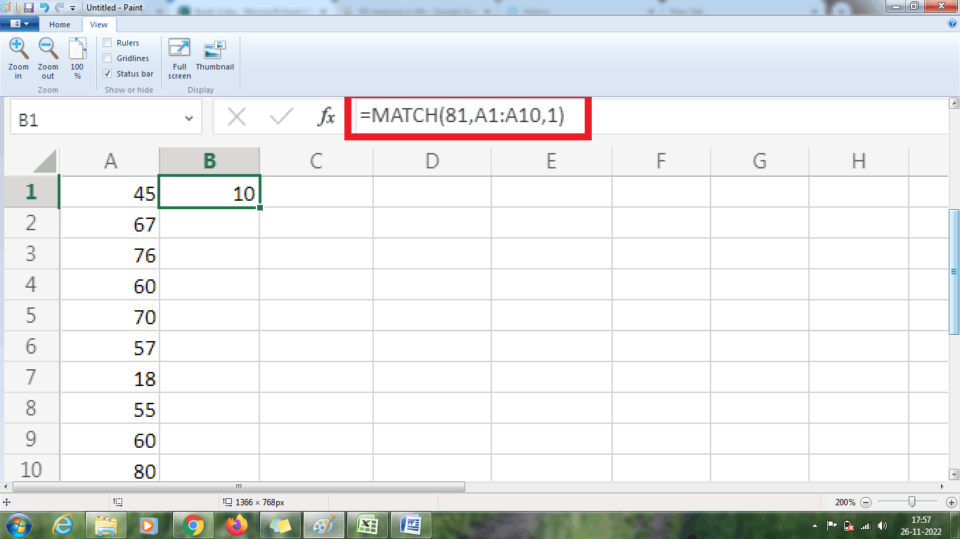
From the above worksheet, the value 81 is not present in the data, hence the MATCH function takes the next value, 80, in the 10th-row position. Hence 10 are displayed as a result in cell B1.
Example 2.3: Find the cell address of the specified data using the formula.
The specified data is found in this example using the formula as=MATCH (81, A1:A10,-1). The steps to be followed are,
Step 1: Enter the range of data in column A1:A10.
Step 2: Select a new cell where the user wants to display the result and type the formula as =MATCH (80, A1:A10,-1)
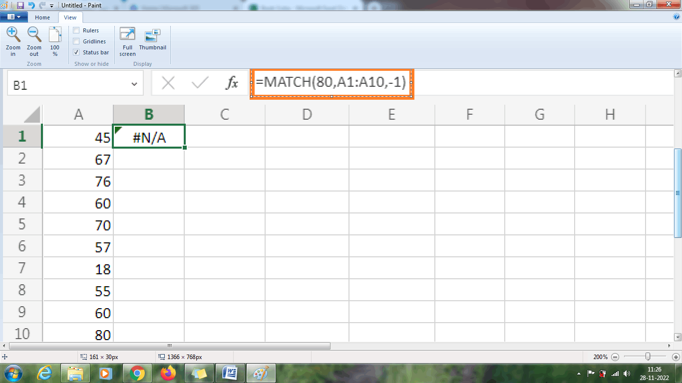
The above worksheet shows the result as an error where the -1 indicates that the value is to be sorted in descending order. But here, the values need to be sorted in descending order. Hence the result is displayed as an error.
Hence, sort the data in descending order and enter the formula as =MATCH (80, A1:A10,-1). The MATCH function will display the exact location of the specified data as follows.
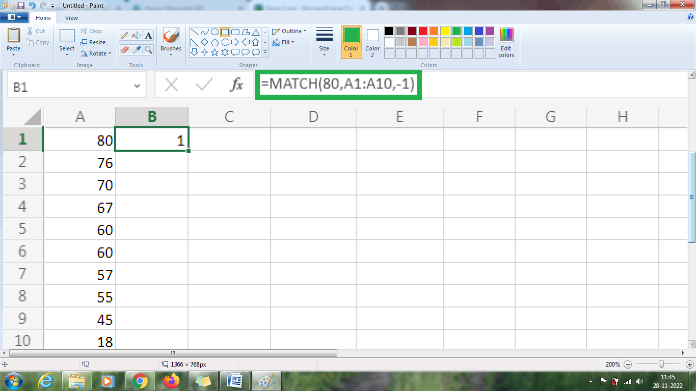
The above worksheet will display the result as 1, which is the location of the data 80.
ADDRESS Function
The address function returns the address of the specified cell.
Syntax
ADDRESS (row_num, column_num,[abs_num],[a1],[sheet text])
row_num – A numeric value indicates the row number used in the cell reference.
column_num – It is a numeric value that indicates the column number used in the cell reference.
abs_num – It is an optional one that is used to specify the type of reference to return.
Example 3: How to retrieve the cell address of the maximum value in the given data?
The ADDRESS function is used along with the MATCH and MAX functions to retrieve the cell address of the maximum value. The steps to be followed are,
Step 1: Enter the range of data in column A1:A10.
Step 2: Select a new cell where the user wants to display the result and type the formula as = ADDRESS (MATCH (MAX (A: A), A: A, 0), 1)
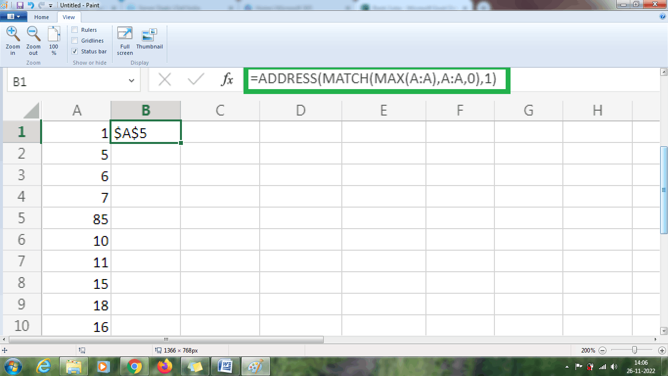
From the above worksheet, the largest value is 85, and the ADDRESS function displays the cell address as $A$5. The ADDRESS function retrieves the data as ADDRESS (5, 1).
Example 4: How to display cell address $D$5 using the ADDRESS Function?
To display the cell value, $D$5, using the ADDRESS function, the steps to be followed are,
Step 1: Enter the range of data in column A1:A10.
Step 2: Select a new cell where the user wants to display the result and type the formula as =ADDRESS (5, 4). Here 5 and 4 indicate the fifth row and fourth column.
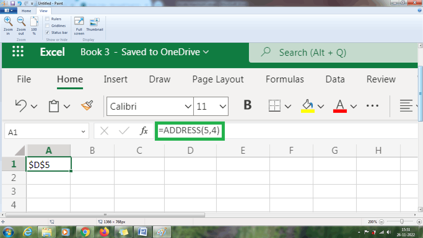
From the above worksheet, the ADDRESS (5, 4) represents the cell value as $D$5.
Example 5: How to display the cell address C$2 using absolute reference?
The absolute reference is used along with the ADDRESS function to indicate the cell address. The steps to be followed are,
Step 1: Enter the range of data in column A1:A10.
Step 2: Select a new cell where the user wants to display the result and type the formula as =ADDRESS (2, 3, 2). Here two and three represent the second row and third column.
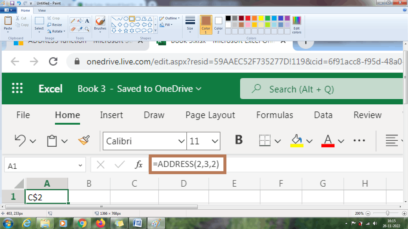
From the above worksheet, the ADDRESS function (2, 3, 2) displays the cell address as C$2.
Summary
From the above worksheet, the various functions and methods to locate the maximum value are explained briefly.