Frequency Distribution in Excel

The term Frequency Distribution in Microsoft Excel is mainly used to explain how the data will be spread out. And it could be achieved with the help of the Histogram, which eventually provides an excellent vision of how the respective data will be distributed.

And to create the Frequency Distribution in Microsoft Excel, an individual must have an "Analysis Toolpak" that can be activated from the ADD-Ins Option available in the Developer menu tab. And once it gets started, an individual needs to select the respective Histogram from the given Data Analysis and then select the data that they need to project effectively.

The Formula for Frequency in the Microsoft Excel

The Formula that is related to the Frequency is mentioned below:

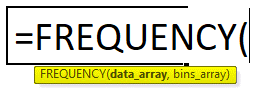
Besides these, the respective Frequency function has two arguments which are as follows:

1. Data Array: A data array is termed to be the set of array values that can be used to count the frequencies, and if the data values are zero, that is, the Null Values, then, in that case, the respective frequency function in the Microsoft Excel primarily returns the array of zero values effectively.
2.  Bins Array: Bins array is the set of the array values used to group the values in the data array. And if the Bin array values are zero having NULKLL VALUES, then in that case, it will return the array elements from the array of the data.

How to Make Frequency Distribution in Microsoft Excel?

The Frequency Distribution in Microsoft Excel is effortless to use; in these, we will understand the working of the Microsoft Excel Frequency Distribution with the help of the various examples discussed below.

It was known that in Microsoft Excel, we could effectively find out the "Frequency function" function in the menu called Formula Menu that comes under the statistical category, with the help of the following steps mentioned below.

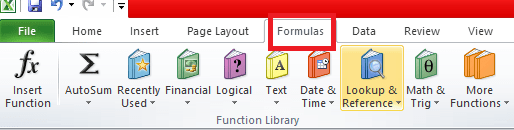
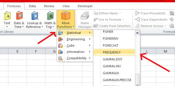
Step 1: First of all, we need to move to the menu that is FORMULA menu, As depicted in the below-attached Screenshot.

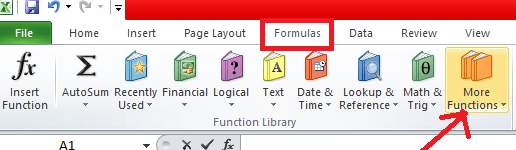
Step 2: Now, we will click on the "More function" options under the Formula. As depicted in the below-attached Screenshot.

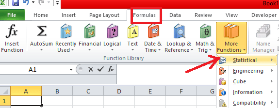
Step 3: After that, under the particular statistical category, we will now choose the "Frequency Distribution" as mentioned in the below-attached Screenshot.

Step 4: After performing the above steps, we will get the Frequency Function Dailaogue box as depicted in the attached Screenshot below. As shown in the below-attached Screenshot.

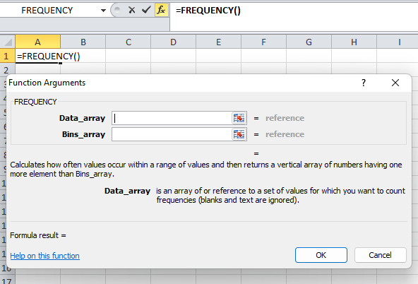
From the above figure, we can say that the data _array or the set of respective values in which we can count the frequencies. In the Bins_ collection, it is considered the array, or we can say it is the set of values where we can effectively group the values in the data array.

#Example 1:

In this particular example, we will be discussing and will see how to find the Frequency for the given or available data set related to the students.

Let’s now consider the below-mentioned example, which will show the score of the Students respectively.

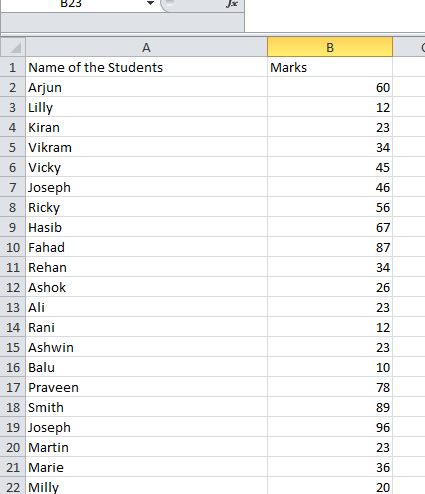
Now, to calculate the Frequency, we need to group the respective data with the students' marks, as depicted in the below-attached Screenshot.

Now, after that, we will be using the frequency functions, and for this, we will group the data with the help of the below-mentioned steps:

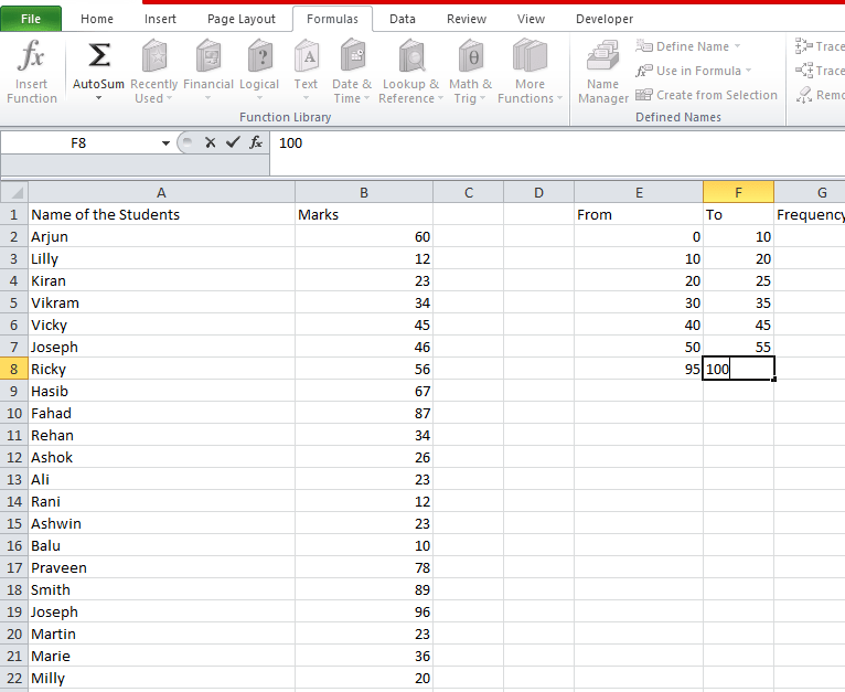
Step 1: In the very first step, we will create a new column named the Frequency.

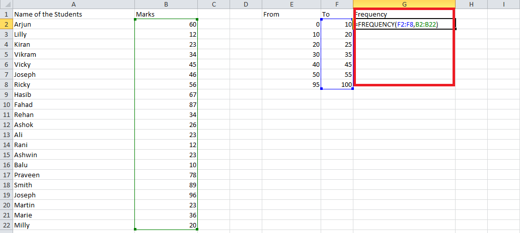
Step 2: Now, after that, we will use the frequency formulation on Column G by effectively selecting columns G3 to G9, respectively.

As shown below in the attached Screenshot.

Step 3: Now, after that, we need to make the selection of the whole frequency column, and then only the frequency function will be able to work efficiently, or else we can get the value that is incorrect to the data (means we will get incorrect output or the result).

Step 4: After that, as per the above-attached Screenshot, it is seen that we have selected the column as per the data array as well as the Bin array as the Students marks =FREQUENCY (F2:F8, B2:B22), and then we will go for the CTRL+SHIFT+ENTER altogether.

Step 5: We can effectively get the desired values in the selected columns.

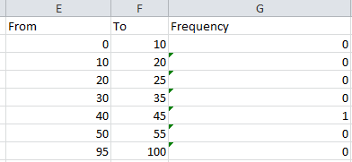
Step 6: Now, once we hit the CTRL+SHIFT+ENTER altogether, we can efficiently see the closing and open parenthesis, as depicted in the Screenshot below.

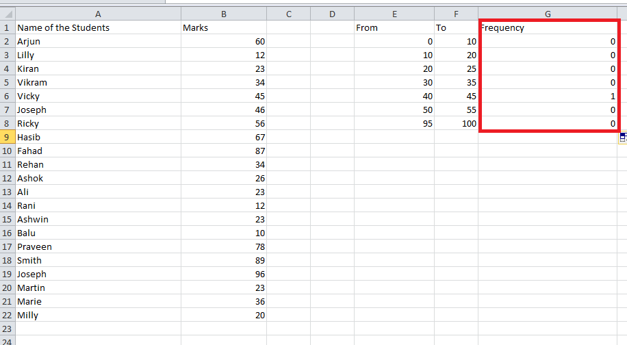
Now with the help of the Microsoft Excel Frequency Distribution, we have efficiently grouped the data of the student's marks, with the marking wise that shows the students has respectively scored the spots in between of the 0-10 we have 0 students, 20-25 we have 0 students and so on as depicted in the below-mentioned figure.

# Example 2: Frequency distribution in Excel with the help of the Pivot Table

In the respective example, we will show how to make the Microsoft Excel frequency distribution with the help of the graphical data via the availability of the database related to sales.

And one of the standards and easiest ways to create (making) the excel frequency distribution is with the help of the pivot table so that we can easily make the graphical data respectively.

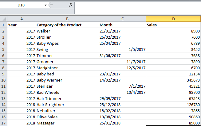
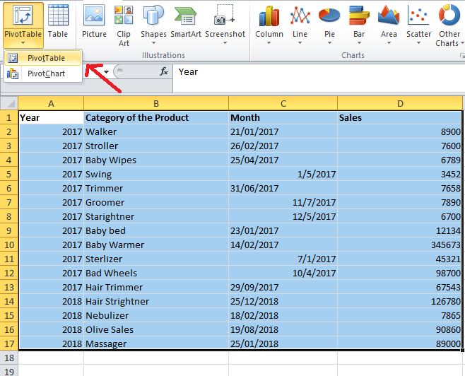
Let us now consider the sales data mentioned below in the attached figure, primarily depicted with the year-wise sales. And with these data, we will see how to use the pivot table with the help of the following steps below.

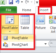
Step 1: First, we need to create the Pivot Table for those mentioned earlier and attach data related to the product sales. And for designing the pivot table, we need to go to the "Insert Menu", and then from that menu, we will select the Option that is the pivot table. As seen in the below-attached Screenshot.

Step 2: Now, after that, we will drag down the sales in the respective Row Labels and then we will drag down the same values of the sales, as depicted in the below-attached Screenshot.

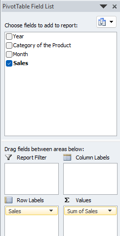
Step 3: Now, in these steps, we will ensure that we have selected the respective pivot field, setting it the sum to get the sum of the sales.

As depicted in the below-attached figure.

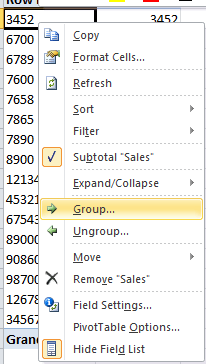
Step 4: Now, after that, we will click on the row label sales number, and then we will right-click and will "Choose the Group Option." As clearly seen in the below-mentioned Screenshot.

Step 5: After performing the above steps, we will encounter the particular grouping dialogue box, as depicted clearly in the attached image below.

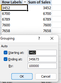
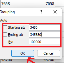
Step 6: Now, after that, we will perform some specific operations on it; that is, we will effectively change the starting from the number 3450 and ending at 345680, and it is Grouped By 100000, and then we will click on the "Ok" button as seen in the below-attached Screenshot respectively.

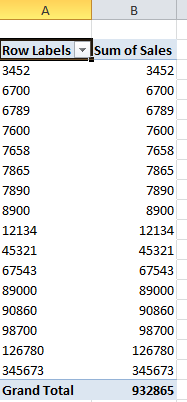
Step 7: After that, we will get the outcome, as shown below in the attached Screenshot.

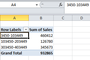
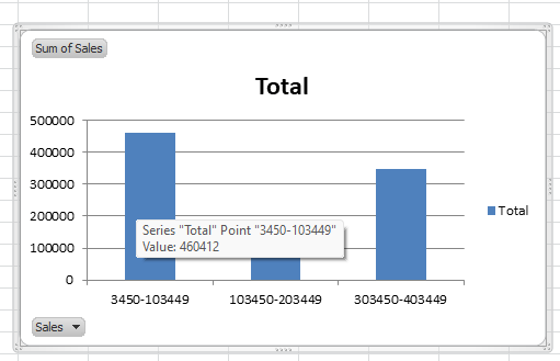
We can see in the above data that the Sales Data is grouped by 100000 with the minimum to the maximum values effectively, which can be shown more professionally by displaying it with the help of the graphical format.

• First, we need to move to the "Insert Menu" and select the Column Chart, as seen in the attached figure below.

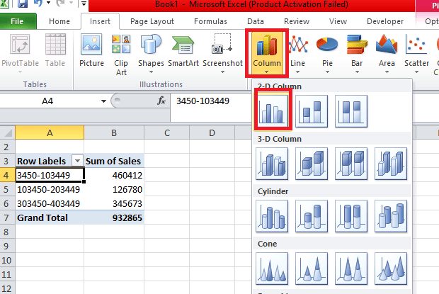
• Now we will get the outcome or the output as follows:

# Example 3: Excel Frequency Distribution with the help of the Histogram

With the help of the pivot table, we need to group the sales data. We will efficiently see how to make out the historical sales data with the help of the Frequency Distribution in Microsoft Excel.

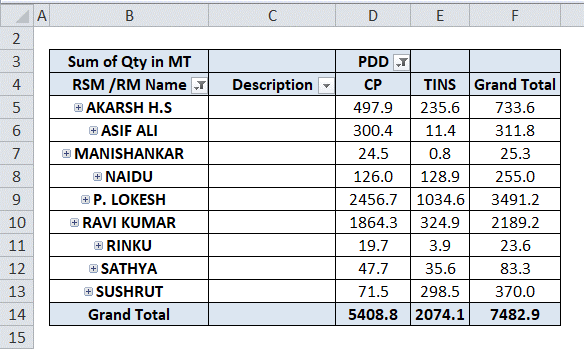
Let us now consider the below sales mentioned sales data for creating the particular Histogram with the Sales Person Name with the corresponding sales value.

The CP is nothing but the consumer pack as well as the Tins are the range values that are how much tins have effectively been sold out for the specific sales persons.

As depicted in the below-attached Screenshot.

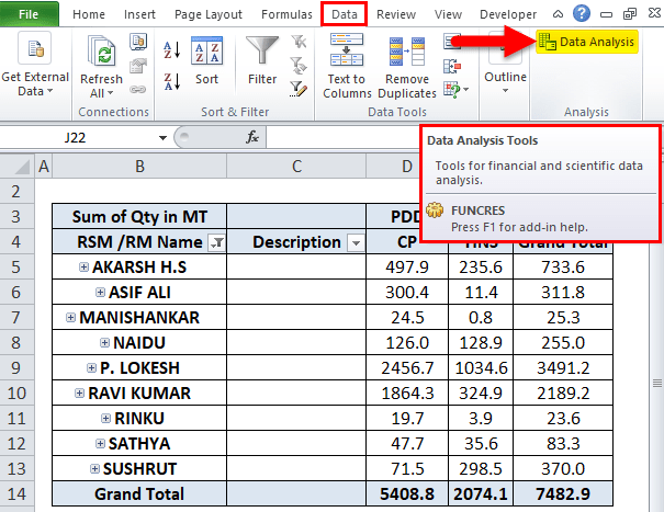
We can easily find the Histogram in the respective data analysis group under the menu of the data, which is nothing but just the add-ins. Now we will see how to apply the Histogram with the help of the following steps.

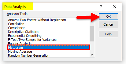
Step 1: First, we will go to the Data Menu at the top of the menu. We can easily find the data analysis, and we will now click on the study of the highlighted data, as depicted in the Screenshot below.

Step 2: After performing the above steps, we will get the dialogue box and then in that, we will choose the Histogram options and click on the "Ok" Button. As depicted in the below-mentioned Screenshot.

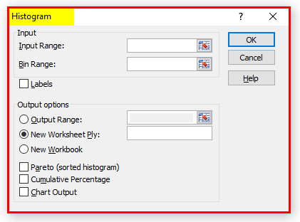
Step 3: We will get out the histogram dialogue box below, as seen in the attached figure.

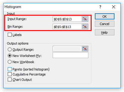
Step 4: After that, we will give the Input Range and Bin Range, as seen in the attached figure below.

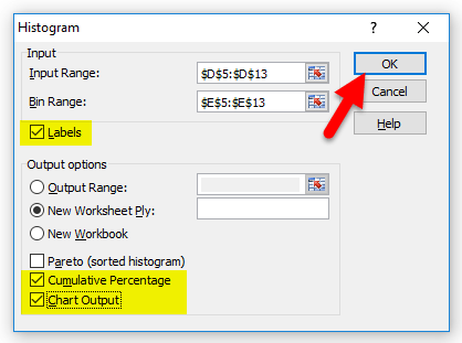
Step 5: Now, we will ensure that we will have a checkmark on all the options, such as label options, chart output, and Cumulative Percentage, and then we will click on the "Ok" button. As seen in the below-attached Screenshot.

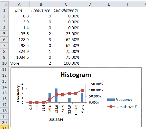
Step 6: After that, in the below chart, we got the respective output that will show the cumulative percentage along with the frequency help. As depicted below Screenshot.

Important Things need to Remember about the Excel Frequency Distribution.

The essential things that need to be remembered by an individual while working on Excel for the frequency distribution on the Excel sheet are as follows:

1. In the respective Microsoft Excel Frequency Distribution, while grouping the data, we might lose some of the critical data, so an individual should make sure that an individual need to group it correctly.
2. While the help of the Excel Frequency Distribution, it should be made sure that the classes must be equal in size with the upper limit and lower limit values, respectively.