Microsoft Excel is used to perform calculations for multiple purposes. The data entered in the worksheet is a combination of numeric and alphabets. Sometimes there is a need to check the number of characters in the cell. Excel provides a default function called LEN, which counts letters, numeric values, characters and spaces. In this tutorial, the steps to count the characters are explained briefly.

1. How to count the characters in the cell?

To count the characters, steps to be followed are:

Step 1: Enter the data in the respective cell.

Step 2: Select the cell, where the result to be displayed. Here cell B1 is selected.

Step 3: In cell B1, enter the formula as =LEN (A1). Here A1 is the cell containing data.

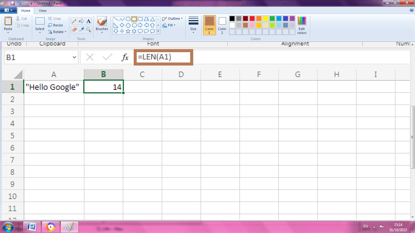
In the above spreadsheet, the formula counts the exact characters in cell A1 including apostrophe marks. “Hello Google” contains exactly fourteen characters, and the LEN function includes 11 letters, 1 space and two sets of the apostrophe.

2. How to count the characters in the range of cells?

To count the characters in the range of cells SUM and LEN function is used. The steps to be followed are,

Step 1: Enter the data in the respective row or columns. Here the data are entered in the cell range from A1:A5

Step 2: Select the new cell, where you want to display the result. Here the cell A6 is selected.

Step 3: Enter the formula in the cell A6 as =SUM(LEN(A1)+LEN(A2)+LEN(A3)+LEN(A4)+LEN(A5)). A1 to A5 are described as data range. The data range can be changed based upon the data entered in the cell.

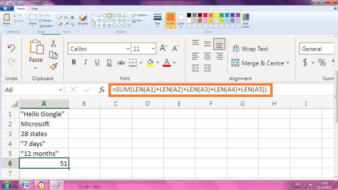
From the worksheet, the total character present in the data range including spaces, apostrophe, numeric and alphabet values from A1:A5 are 51 which is calculated using the function called LEN and SUM.

3. How to count the range of cells using array formula?

An alternative method to count the range of cells is using an array formula. Using the default formula is a longer one.

The steps to be followed are,

Step 1: Enter the data in the spreadsheet. Here the data are entered in range from A1:A5.

Step 2: Select the new cell, where you want to display the result. Here the cell B1 is selected.

Step 3: Enter the formula in the cell B1 as, =SUM (LEN (A1:A5)). Here A1:A5 is called cell range.

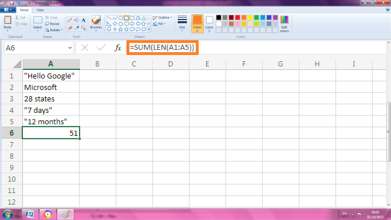
From the above worksheet, the data range A1:A5 is calculated using the array formula. The array constant {14, 9, 9, 8, 11} is used as an argument for the SUM function. The result is displayed as 51 which count the exact characters in the selected cell.

This formula is simply works in Excel 365 or Excel 2021. One can press Enter key after finish typing the formula. For prior versions, press CTRL+SHIFT+ENTER. A curly brace will present in the formula.

4. How to count the specific characters in the cell?

Sometimes, there is a need to count the specific characters in the cell. Excel provides the default function called “SUBSTITUTE” and “LEN” which calculates the specific characters in the cell. The steps to be followed are,

Step 1: Enter the data in the cell. Here the data entered in the cell are A1

Step 2: Select the cell where you want to display the result. Here the cell B1 is selected.

Step 3: In the cell enter the formula as =LEN (A1)-LEN (SUBSTITUTE (A1,”o”,””)). Here ‘o’ indicates, how many times the letter is repeated.

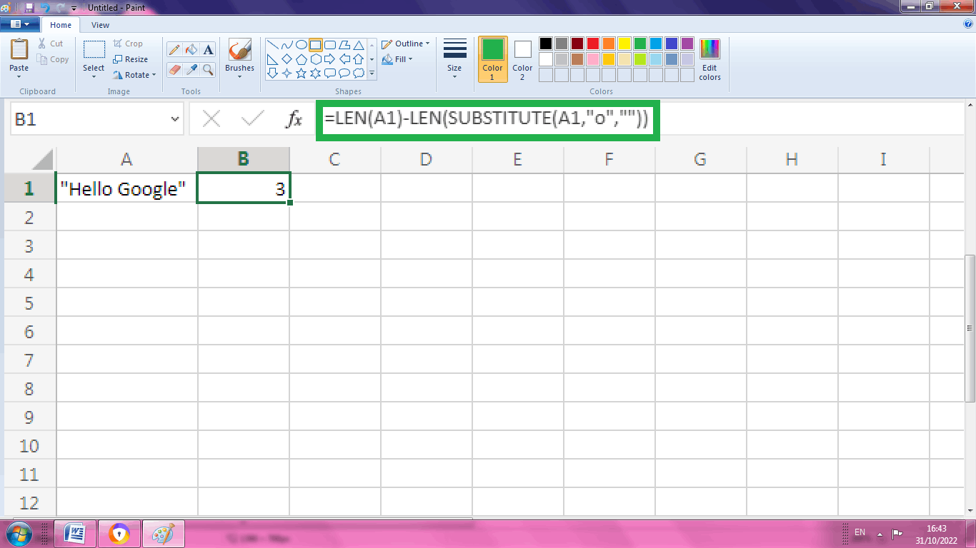
From the above worksheet, the letter “o” is repeated three times. The substitute function is used to replaces the character (second argument) with an empty string (third argument). LEN (SUBSTITUTE (A1,”o”,””)) equals 11. Here “11” is the length of the string without the character o. If 11 is subtracted from 14(total characters present in cell A1), the result is 3. Therefore 3 times the letter o is repeated.

5. How to calculate the specific characters using array formula?

To calculate the specific characters using array formula, the steps to be followed are,

Step 1: Enter the data in the cell range. Here the data are entered in the range A1:A5

Step 2: Select the cell where you want to display the result. Here cell range A6 is selected.

Step 3: Enter the formula in the cell A6 as =SUM (LEN (A1:A5)-LEN (SUBSTITUTE (A1:A5,”a”,””))).

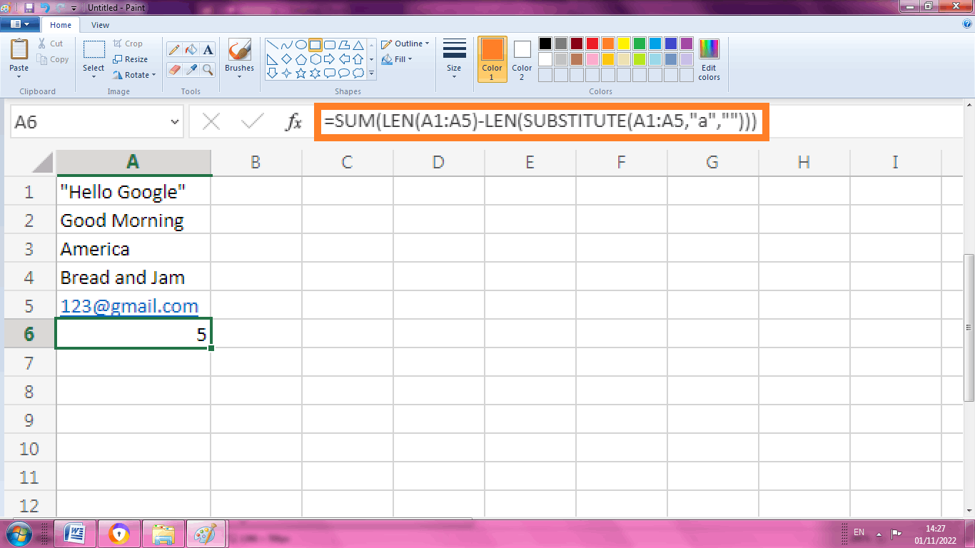
From the above worksheet, the result is displayed as “5” in the cell A6. From the formula the array constant {1, 3, 1} is used as an argument for the SUM function which displays the result as 5. Here the function called SUBSTITUTE is case-sensitive where the capital letter “A” is not selected while counting.

6. How to calculate the lower and uppercase of a Specific character?

To calculate both the lower and upper case in a specific character using array formula, steps to be followed are,

Step 1: Enter the data in the cell range. Here the data are entered in the range A1:A5

Step 2: Select the cell where you want to display the result. Here cell range A6 is selected.

Step 3: Enter the formula in the cell A6 as =SUM (LEN (A1:A5)-LEN (SUBSTITUTE (LOWER (A1:A5),”a”,””))).

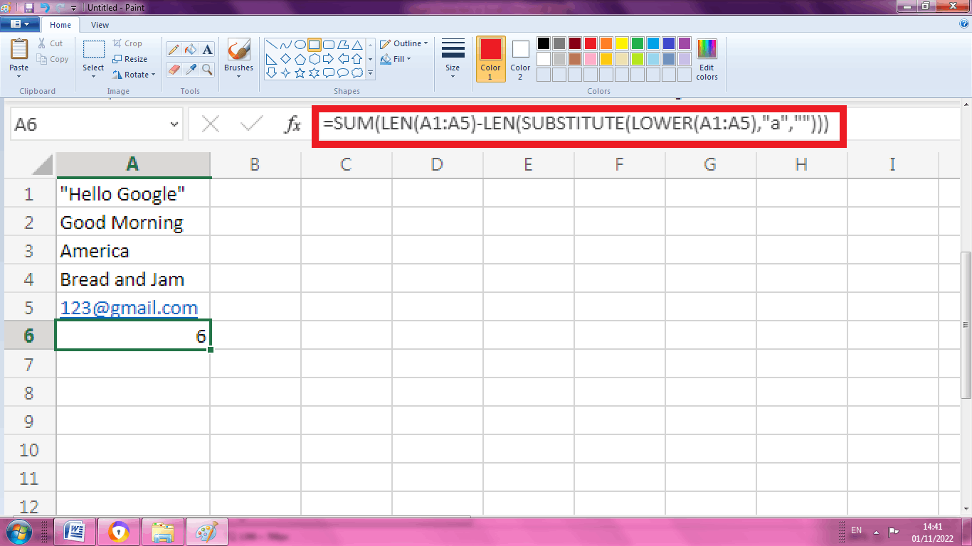
The above worksheet shows the result as “6” in cell A6. The function “LOWER” is used to convert all the letters to lowercase and counts the number of specific characters in the data. The argument {2, 3, 1} is used as an argument for the SUM function.

Summary

From the above tutorial, the various method and functions to count the characters is explained briefly.

Excel Tutorial

Functions

How To

Misc