How to Make Use of the F-Test in Excel

Intro to F-Test in Microsoft Excel

F-Test is primarily considered to be the essential tool of statistical in Microsoft Excel that, in turn, is used to do the hypothesis test with the help of the respective variance of 2 datasets or the populations. And we can be able to calculate whether the Null Hypothesis (H0) for the given set of detailed data is TRUE or not. This can be made sure when the shared variance of both data sets seems to be equal.

Besides all these, in order to perform the respective F-Test, we need to move to the “Data Menu" tab, and from the Data Analysis option, we will select out the F-Test Two Sample of Variances. After that, we need to choose both the Data population in variable 1 and the variable 2 range effectively and keep the Alpha as 0.05 (Standard for the probability Percentage of about 95%). And this will give us the final F-test calculation. If F>F Critical One is Tail, then, in that case, we will reject the Null Hypothesis, which means that the particular selected data population is not equal.

How to do the F-Test in the Microsoft Excel

The F-Test in Microsoft Excel is straightforward to use, and now let's understand the working of the F-test in Microsoft Excel with the help of various examples.

# Example 1: F-Test in the Microsoft Excel

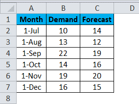
Let us make assumptions that we have 6-months of data on the particular Demand as well as the forecasting of the product. And the Data are given in the A2:C7 respectively.

As clearly depicted in the below-attached screenshot,

And on moving further now, if we need or want to test the variation and the difference in the variability of the data, we need to follow the below-mentioned steps respectively.

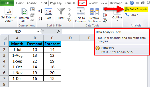
Step 1: First, we need to go to the "Data" in the Menu Bar and then select "Data Analysis," as seen in the screenshot below.

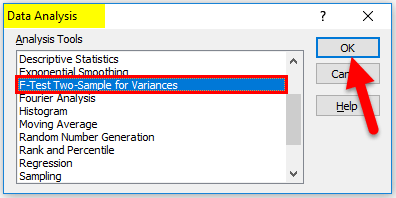
Step 2: And in these steps, when we once click on it, then a Data Analysis option box will appear on the screen, and now we will select the "F-Test Two-Sample Variances", and then we will click on the "Ok" button. As it is depicted in the below-attached screenshot,

Step 3: After that, we will encounter the other dialogue box of the F-Test, as seen in the below-attached screenshot.

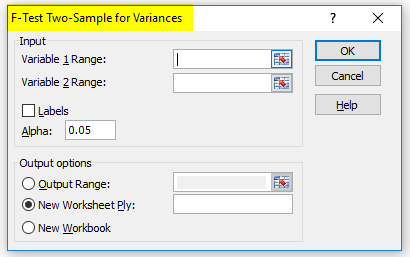
Step 4: Now here, we need to select the variable range of the Demand and the Forecasting from the respective Data; that area is effectively shown in the below-attached screenshot.

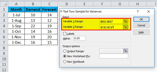
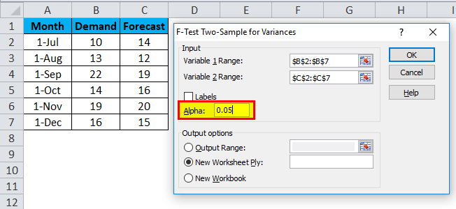
Step 5: Now, after making the selection of the Variables 1 Range as well as the Variables 2 Range, we will then choose the desired value of the Alpha in the same box respectively, and here in these, we have taken the "0.05" as Alpha, that means we are primarily considering out the 5% of the tolerance in the calculation as well as in the analysis, as we can see in the below-attached screenshot.

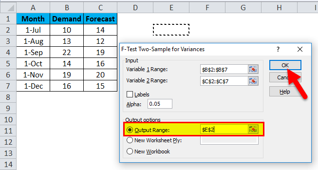
Step 6: Soon after performing the above operations, after that, we will be selecting the "Output Range" cell anywhere in the same excel sheet or else, we can make a selection of the New Workbook as well, which is given just below it respectively for our ease. And in these, we have created a section of the output range as "E2", and then we will click on the "Ok" button.

As is depicted in the below-attached screenshot effectively,

Step 7: The respective F-Test in Microsoft Excel will look like this, as seen in the screenshot below.

Now, after that, we will analyze the above data,

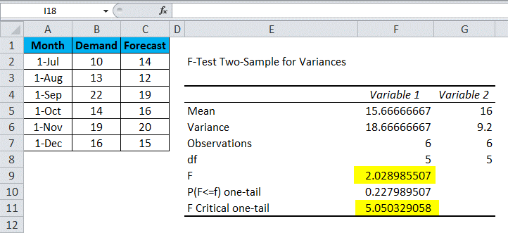
1. The Mean: The Mean of variable 1 and the Mean of variable 2 are 15.66666667 and 16 effectively, the mid-point of the Demand and the Forecasting.
2. A variance: The variances of variable 1 and variable 2 are 18.66666667 and 9.2, effectively showing the variation in the particular data set.
3. Observations: The Observations of variable 1 and the observations of variable 2 are none other than the 6, which means 6 data points or the parameters considered in the F-Test, respectively.
4. df: The df is considered to be the Degree of the Freedom, that area shown only for the 5 variables that can be assigned to this particular statistical distribution.
5. P (F<=f) one-tail: The P (F<=f) one-tail is defined to be the probability distribution of the variations in both datasets that are coming to be the approximation of 22.7%.

From the above, we can clearly see that the value for the F is 2.02898507, which is primarily lesser than the value of the F Critical one-tail, meaning that the Null Hypothesis can be accepted respectively.

#Example 2: F-Test in the Microsoft Excel

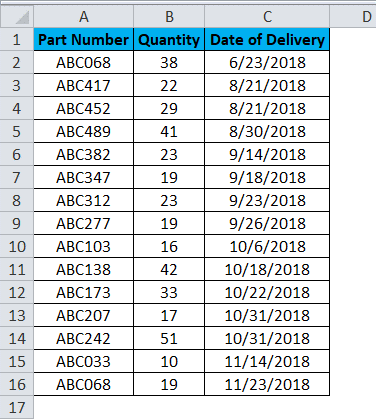
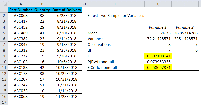
Let us now assume that we have encountered some part numbers' delivery data. To better understand, we have efficiently sorted out the data in ascending order with the respective column name and the Date of Delivery, as shown in the screenshot below.

Moving further, we will follow the same process for this data to perform the F-Test in Excel. The Data set has only one column with the statistical and the numeric value or the figures. Here, the detailed analysis will be based on effectively segmenting the particular dates in the two sections. As it is seen in the below-attached screenshot,

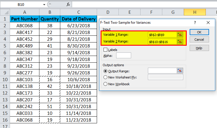
Step 1: As seen in the below-attached screenshot, the Variable 1 Range data is selected from the cell that is from B2:B9, and the Variable 2 Range data is selected from the cell from B10:B16.

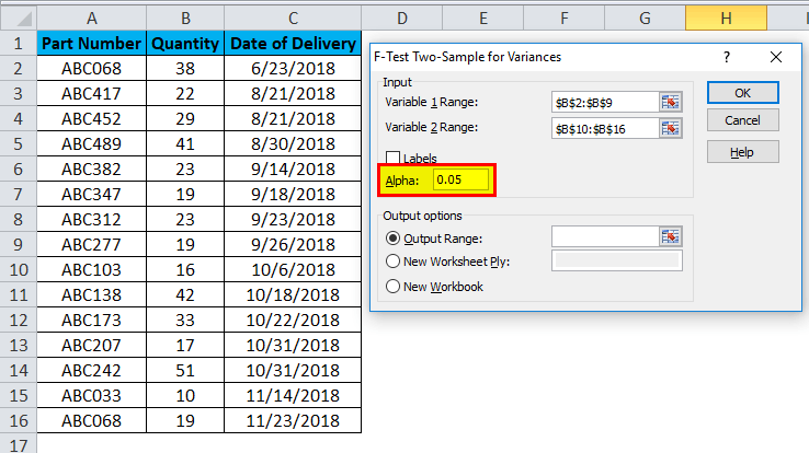
Step 2: And the Alpha is kept at "0.05", which is 5% of the tolerance (We can effectively change the value of the Alpha as per the requirement and as per the need of the data size). As was seen in the below-attached screenshot,

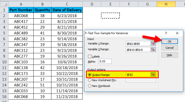
Step 3: Then after that, in this step, we will be selecting out the "Output Range" cell, and then we will click on the "Ok" button, as it is depicted in the below-attached screenshot.

Step 4: The F-Test in Microsoft Excel for the Delivery Data of the respective shown Part Numbers will look like this, as seen in the screenshot below.

Now we will be analyzing the above data in detail,

1.  The Mean: In the above example, the Mean of the particular Variable 1 and Variable 2 are 26.75 and 36.85714286, effectively considered to be the mid-point of the Quantity Delivered. And it was under the noticed that there is not much amount of the difference in these parameters.
2. A variance: In these examples, the variance of variable one and variable 2 are 72.21428571 and 235.1428571, respectively, which primarily shows the variation in the given dataset.
3. Observations: The observations for the above discussed example, the Variable 1 and variable 2 are 8 and 7, which means that the selected upper data points are 8. And similarly, the selected lower points are 7 in the numbers respectively.
4. df: The df is termed the Degree of Freedom as shown. The only value that 7 and 6 variables are effectively assigned to the respective upper and the lower data set in this particular statistical distribution.
5. P (F<=f) one-tail: The P (F<=f) one-tail is defined to be the probability distribution of the variations in both the data sets, which comes as 0.073953335 (7.3% approximately).

From the above discussion, we have seen that the value of F is usually 0.307108141, that in turn seems to be the greater than the value of the F Critical one-tail, this will indicates that it could be the the Null Hypothesis and these cannot be accepted in any circumstances.

Pros Side of the F-Test in the Microsoft Excel

The various pros side of the respective F-Test in the Microsoft Excel area follows:

1. The F-Test can be effectively used in any statistical data set in which the comparison of before or After, Latest,/Previous can be performed to accept if the statistical data is accepted or rejected.
2. And the particular Mean gives out the mid-value, which can be considered the average of the total values, And the Variance gives out the difference between the actual and the predicated/future value so that the centricity can be effectively seen straightforwardly without facing any of the difficulties.

Cons Side of the F-Test in the Microsoft Excel

The various cons side of the respective F-test in Microsoft Excel is as follows:

1. It was known that for an un-statistical background, it is a little bit difficult to understand and measure the different observations respectively.
2. And the other cons of the F-Test in Microsoft Excel is that there are tiny differences in the F and F, Critical one-tail values. Then it becomes very much challenging in order to accept as well as to make rejection of the test while performing this particular test in the real-life scenarios.

Things to remember

The Following things need to be remembered by an individual while working with the F-Test in Microsoft Excel are as follows:

1. It must be kept in mind that, F-Test can be effectively performed on one or more sets of detailed data in Microsoft Excel and is not restricted to the data set with two parameters.
2. And the other point is that an individual must needs to make sorting of the just data before performing of the particular F-Test in Microsoft Excel, and the sorting parameter should be considered as the base which is then correlated with the respective data efficiently.
3. And last but not least, an individual needs to do the basic formatting before performing the F-Test to get the sound-sanitized output.