Conditional Formatting in Excel

Conditional Formatting

What are the conditional formats?

Conditional Formatting is a tool that allows the user to format cells or range of cells based on the selected condition or given criteria. The formatting will keep changing depending on the value of the cell or formula returning value. Conditional Formats apply formats to cells bases on the value in the cell or a group of cells.

Different ways to use Conditional Formatting

Highlight Cells Rules

It is used to highlight the cells based on their values. You can also apply the format on one cell first and then copy the format on other cells using ‘Format Painter’.

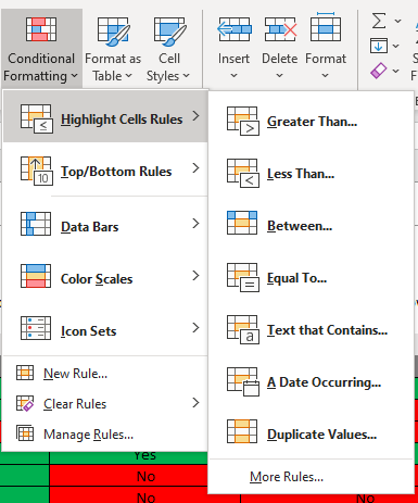
• Greater Than – it will highlight all the selected cells which are above a particular value – you can change the value depending upon what you want and can also change the colour with which you want to highlight the cell
• Less Than – it will highlight all the selected cells which are below a particular value – you can change the value depending upon what you want and can also change the colour with which you want to highlight the cell
• Between – it will highlight all the selected cells which are above between 2 specified values – you can change the values depending upon what you want and can also change the colour with which you want to highlight the cell
• Equal to – it will highlight all the selected cells where the value is equal to a specified value – you can change the value depending upon what you want and can also change the colour with which you want to highlight the cell
• A Text that contains – it will highlight all the selected cells which contain a specific text – it can be a name, a letter, alphanumeric values like combination of numbers and alphabets – you can change the values depending upon what you want and can also change the colour with which you want to highlight the cell
• A Date Occurring– used for cells consisting of dates - it will highlight all the selected cells where the date falls in one of the options in the drop-down list – yesterday, today, tomorrow, last month, next month, etc.
• Duplicate Values – It will highlight the cells which have duplicate values or unique values from a group of cells.

Example 1

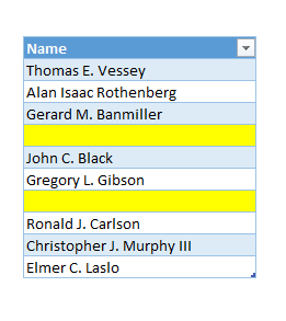
Objective: Highlight the empty cells in the 'Name' column with yellow color

Name

Thomas E. Vessey

Alan Isaac Rothenberg

Gerard M. Banmiller

John C. Black

Gregory L. Gibson

Ronald J. Carlson

Christopher J. Murphy III

Elmer C. Laslo

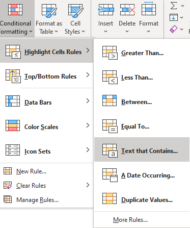
Step 1: Select the data. And click on Conditional Formatting-> Highlight Cells Rules-> Text that contains

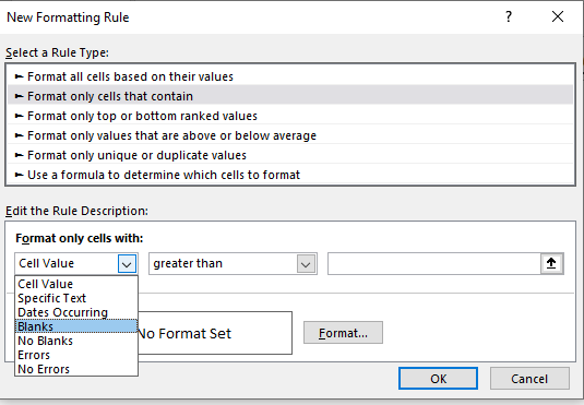
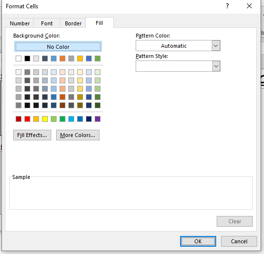
Step 2: From the cell value dialogue box, select the blank option.

Step: 3 The next step is to click on the formal option and fill the yellow colour.

Step 4: Click on Ok. You will notice, the blank cells have been formatted with yellow colour.

Output

Example 2

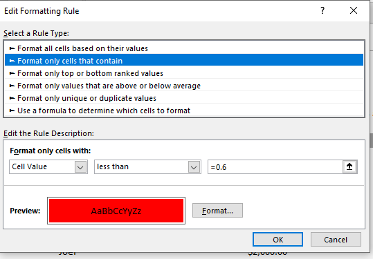
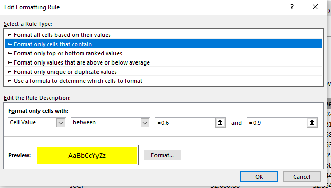
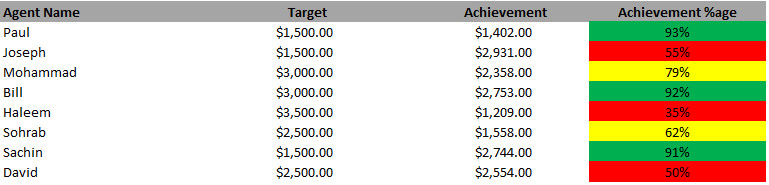
Objective: Prepare a report, in which we want see 90% and above in "green", 60% - 90% in "Yellow" and below to 60% in "Red"

Agent Name	Target	Achievement	Achievement %age
Connor	$2,000.00	$1,402.00	91%
Hall	$1,500.00	$2,931.00	55%
Bruno	$3,000.00	$2,358.00	79%
Stuart	$3,000.00	$2,753.00	92%
Craig	$3,500.00	$1,209.00	35%
Hiram	$2,500.00	$1,558.00	62%
Brenden	$1,500.00	$2,744.00	91%

Step 1: Select Conditional formatting-> Highlight Cell Rules -> less than

Step 2: Select Conditional formatting-> Highlight Cell Rules -> between

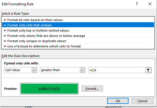
Step 3: Select Conditional formatting-> Highlight Cell Rules -> greater than

Output

Top/Bottom Rules

Top/ Bottom rules in conditional formatting is used to highlight cells based upon values of a group of cells and not just one cell. This formatting option is only used for cell consisting of numbers.

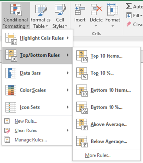
• ‘Top 10 Items’ – It highlights the top 10 cells with the largest values. You can change number of items as well along with the colour.
• ‘Top 10%’ – It highlights 10% cells having largest values. So, if there are 100 cells, it will highlight 10 cells with the highest values. You can change percentage of items as well along with the colour.
• ‘Bottom 10 Items’ – It highlights 10 cells with the smallest values. You can change number of items as well along with the colour.
• ‘Bottom 10%’ – It highlights 10% cells based having lowest values. So, if there are 1000 cells, it will highlight 100 cells with the smallest values. You can change percentage of items as well along with the colour.
• ‘Above Average’ – It highlight all cells which have values above average of all the cells. You can change the colour with which you want to highlight the cell.
• ‘Below Average’ – It highlight all cells which have values below average of all the cells. You can change the colour with which you want to highlight the cell.

Example 1

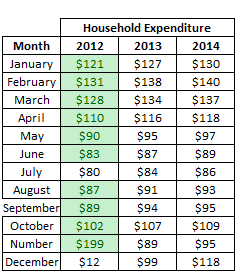
Objective: For year 2012 in the table given below, highlight the top 10 values based on costs using 'Conditional Formatting'.

	Household Expenditure
Month	2012	2013	2014
January	$121	$127	$130
February	$131	$138	$140
March	$128	$134	$137
April	$110	$116	$118
May	$90	$95	$97
June	$83	$87	$89
July	$80	$84	$86
August	$87	$91	$93
September	$89	$94	$95
October	$102	$107	$109
Number	$199	$89	$95
December	$12	$99	$118

Step 1:  Select the entire column for year 2012 and click on Conditional Formatting-> Top/Bottom Rules-> top 10 Items.

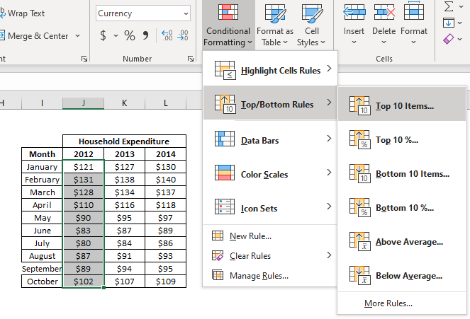
Output

Data Bars

The Data bars option helps in data visualization while working on cells consisting of numbers. It adds bars to individual cells – for a cell containing a large value as compared to other cells, the bar will be broader else it will be shorter. For negative values, the bar will be in the opposite direction of the positive values and usually in a different colour.

Example 1

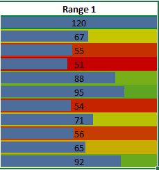
Objectives: Generate random numbers between 50 and 100 and format in Data Bars based on their values.

Range 1
67
55
51
88
95
54
71
56
65
92

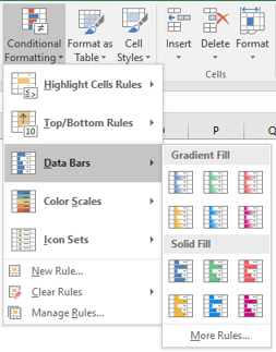
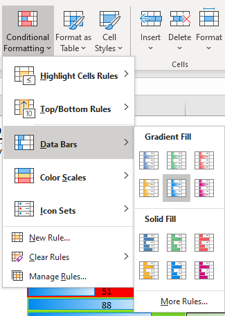
Step 1: Select the data and click on Conditional Formatting-> Data Bars. Select the Gradient Fill or Sold fill colours as per your choice. You will get the below table demonstrated in the output.

Output

Color Scales

This option also helps in data visualization while working on cells consisting of numbers. It can be used to give a 2-colour scale or a 3-colour scale to the group of cells and will keep on changing the colour as we move from one cell to another.

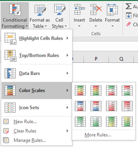
Icon Sets

These are also used for data visualization and are very similar to colour scales.

New Rule

The first five options are what we have mentioned above so far. We will discuss the last option of using a formula.

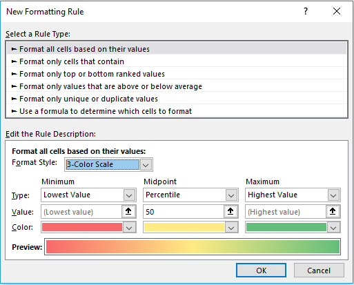
‘Use a formula’ – you can call an excel formula to do conditional formatting.

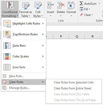
‘Clear Rules’

This can be used to clear the conditional formatting from the selected cell or from the entire worksheet, tables and pivots.

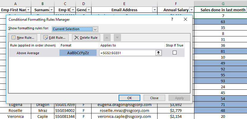
‘Manage Rules’

Helps in editing the existing rules. Go to the cells whose rule you want to edit and click on Manage rules and then you can change the rules.