Division in Excel

Excel worksheet are widely used for calculation purposes. Mathematics calculations include addition, subtraction, multiplication, division etc. Performing this calculation manually takes time and sometimes leads to error. To get the result quickly and efficiently Excel provides some default functions to perform the calculation. Sometimes for several calculations there is no function present in Excel. An alternative method is to use the mathematical symbols or expressions for calculation purposes. Here in this tutorial, the step to perform division is explained clearly.

1. How to divide the value in Excel?

Excel doesn’t provide any default function for dividing the values. In Mathematics the division is performed using the symbol forward slash (/). Similarly in Excel also this method is applicable.

To perform the division the following are the steps:

Step 1: Enter two data in the cell namely A1 and B1.

Step 2: Choose a cell namely C1, to display the result.

Step 3: Enter the formula in the cell C1 as = A1/B1.

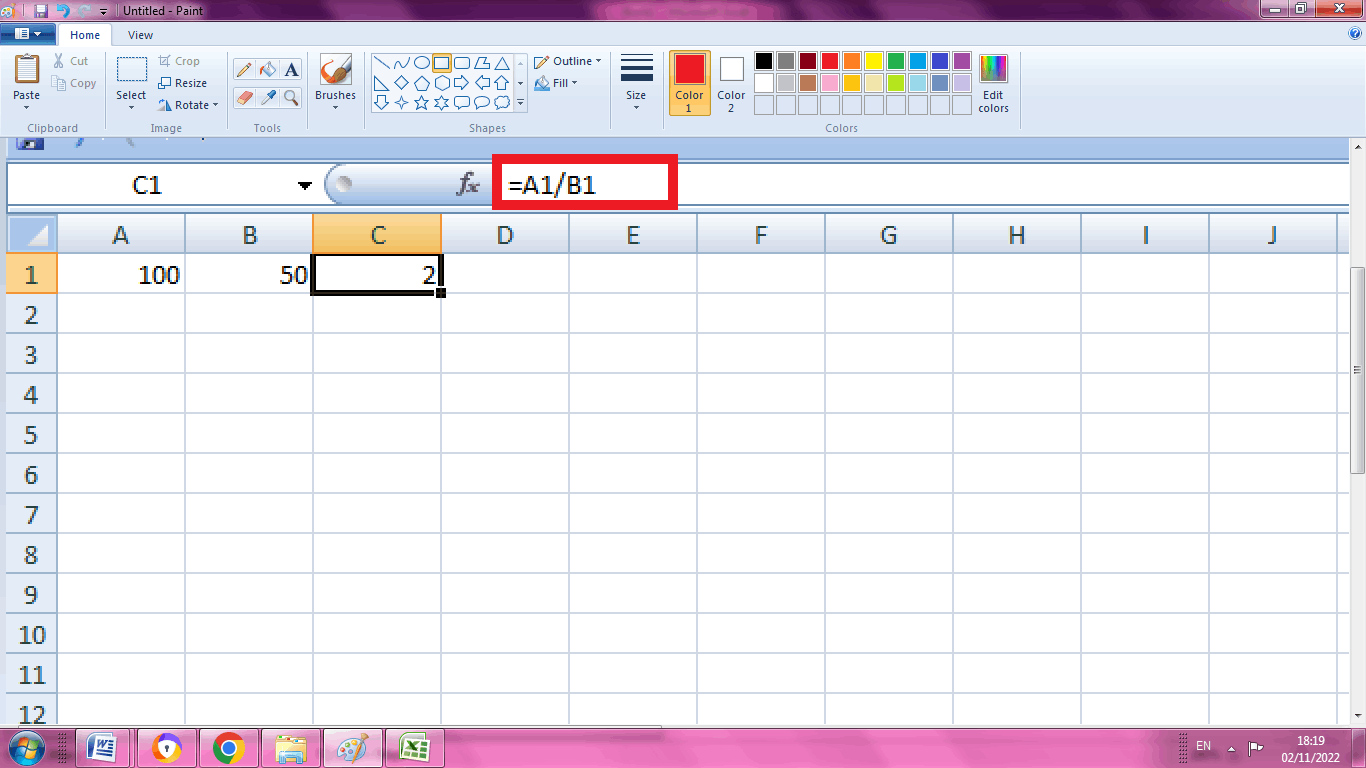
From the above worksheet, the result is displayed in the cell C1.

2. How to divide two numbers directly in Excel?

From the previous concept, the Excel numbers divides the two numbers using cell value. Here, the numbers are divided directly, by the following steps.

Step 1: Enter the two values directly in any cell namely A1, such as =100/5. It should start with ‘=’ sign.

Step 2: Press Enter.

Step 3: The result will be displayed in the cell A1.

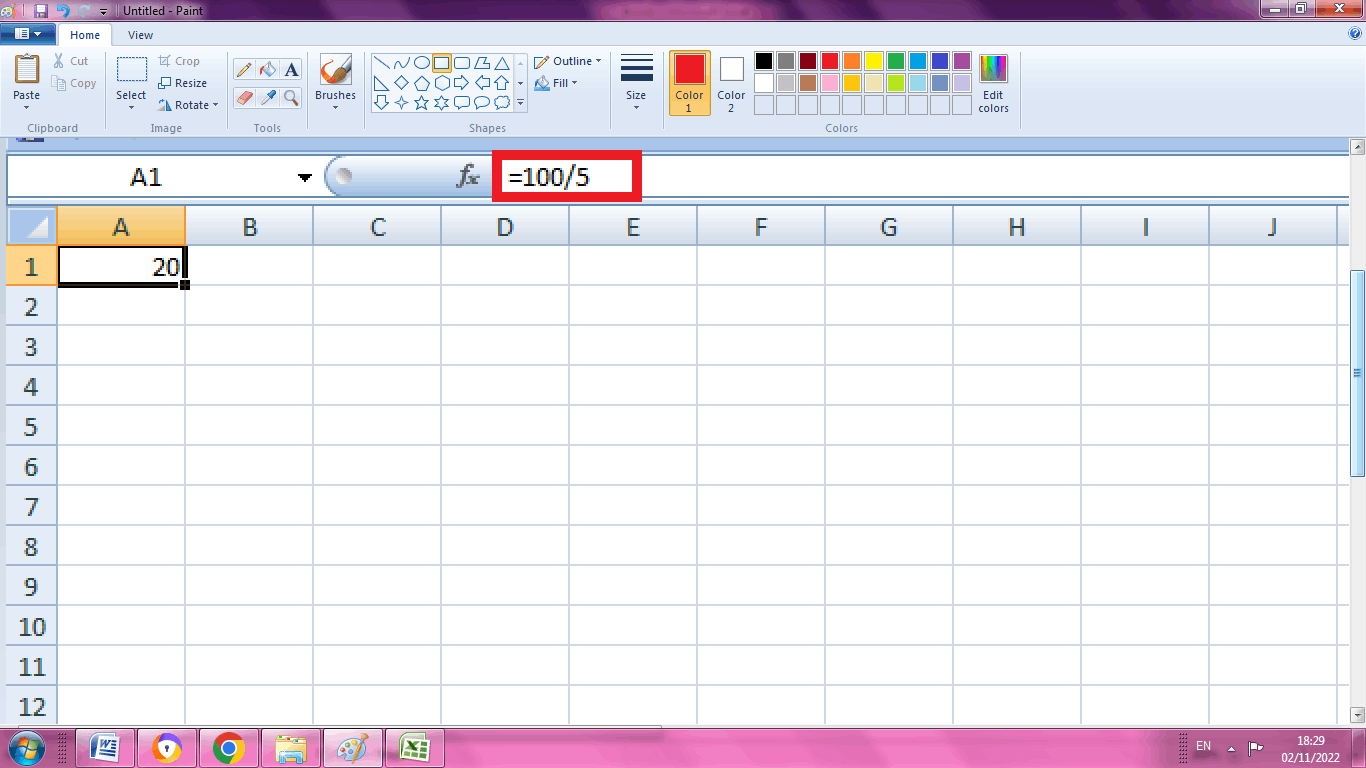
From the above worksheet, the result is displayed in the cell A1.

3. How to get the quotient of the dividing number?

To get the quotient of the dividing number, Excel provides a default function called QUOTIENT which is used to return the quotient of the number. It returns the integer part of the division. It simply eliminates the remainder of a division.

The steps to be followed to use the QUOTIENT function is as follows,

Step 1: Enter two data in the cell namely A1 and B1.

Step 2: Choose a cell namely C1, to display the result.

Step 3: Enter the formula in the cell C1 as = QUOTIENT (A1, B1)

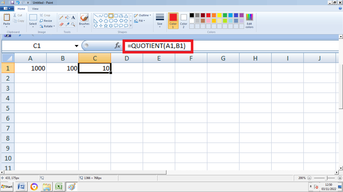
From the above worksheet the result is displayed in the cell C1. C1 contains the quotient of the given value or data.

4. How to get the remainder of the dividing number?

To get the reminder of the dividing number, Excel provides a default function called MOD which is used to return the reminder of the number. It returns the remainder of a division. It simply eliminates the integer part of the division.

The steps to be followed to use the MOD function is as follows,

Step 1: Enter two data in the cell namely A1 and B1.

Step 2: Choose a cell namely C1, to display the result.

Step 3: Enter the formula in the cell C1 as = MOD (A1, B1)

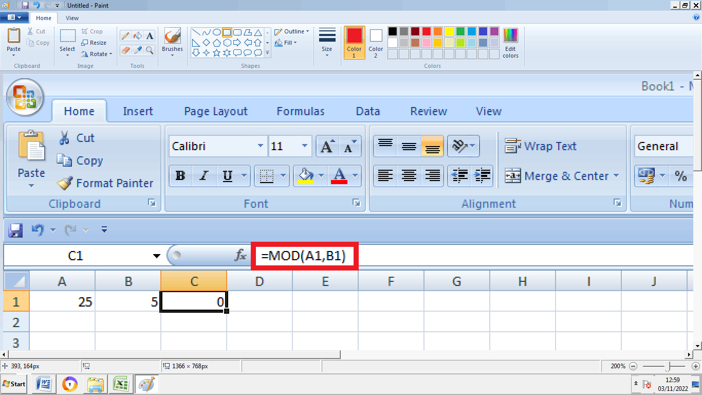
From the above worksheet, the remainder is displayed in the cell C1. The MOD function returns the remainder of the given data.

5. How to divide the two numbers in a range of columns?

To divide the two numbers which is present in the range of columns, the steps to be followed for calculation is,

Step 1: Enter the range of data in the column range A1:B5

Step 2: Choose a cell namely C1, to display the result.

Step 3: Enter the formula in the cell C1 as = A1/B1. The result will be displayed in the cell C1. To get the result of the remaining cell, drag the formula towards the cell B5. The result will be displayed in the remaining cells of data.

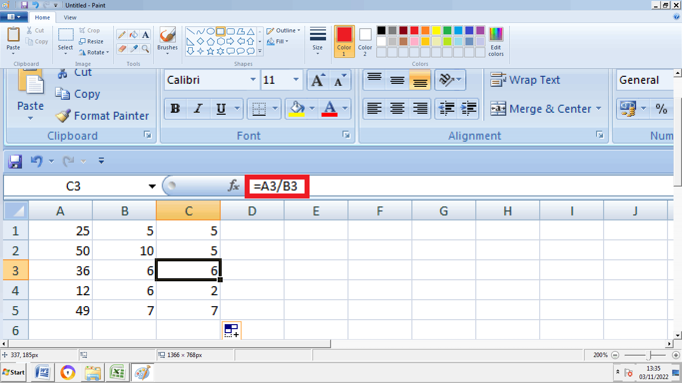
From the above worksheet, the values are present in the column C1:C5 by dragging the formula in the respective cell.

6. How to divide the numbers by a constant number?

To divide the numbers by a constant number, the steps to be followed for calculation is,

Step 1: Enter the range of data in the column range A1:A5

Step 2: Choose a cell namely C1, to set a reference value

Step 3: Enter the formula in the cell B1 as = A1/$B$1. The result will be displayed in the cell B1. To get the result of the remaining cell, drag the formula towards the cell B5. The result will be displayed in the remaining cells of data.

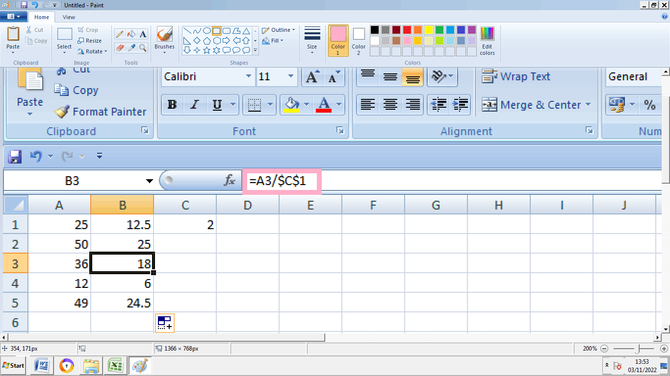
From the above worksheet, the values are displayed in the column range B1:B5 by dragging down the formula. The reference cell value is fixed using the symbol $ in front of the column letter and row number such as ($C$1). While dragging down the formula, the absolute reference ($C$1) won’t change while the relative reference (A1) change according to cell value A2,A3,A4 etc.

7. What is the result of dividing a number with zero or empty cell?

Data is a combination of decimal, numeric, integer, whole number etc. So what is the result if a number is divided with zero or empty cell?   The steps to be followed to check the number are,

Step 1: Enter the data in the cell A1 and A2.

Step 2: Choose a cell namely C1, to display the result

Step 3: Enter the formula in the cell C1 as = A1/B1. The result will be displayed in the cell C1 as #DIV/0! , as the value present in the cell B1 is zero or empty cell.

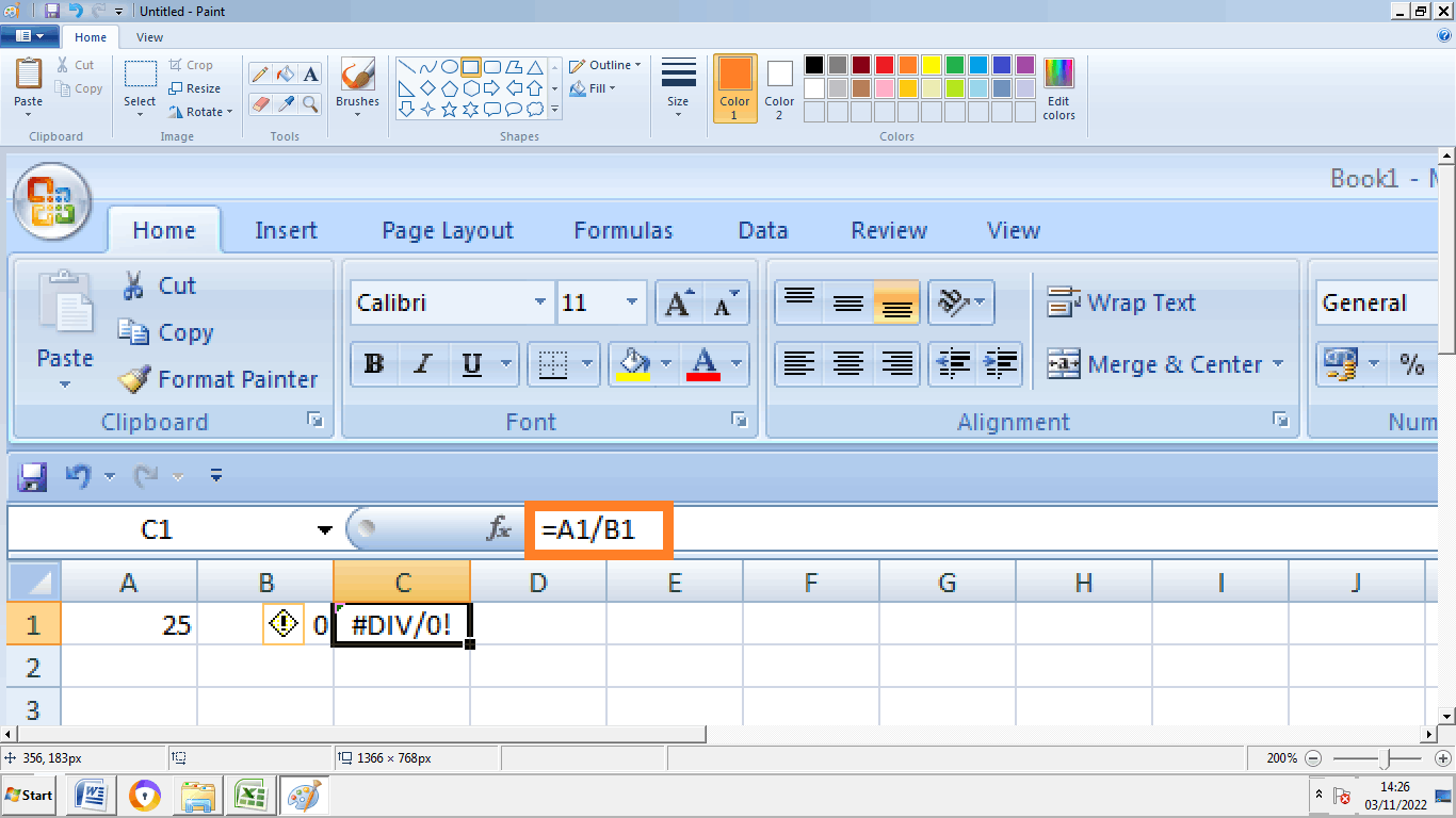
The result is displayed in the cell C1 as shown in the above image.

8. What is the alternative method to divide the number in Excel?

From the previous concept, the number is divided using formulas. Another alternative method to divide the number in Excel is using Excel default function as follows,

Step 1: Enter the range of data in the cell A1:A5

Step 2: Select the cell B1, and enter the value of preference which is the number, divides the value present in column range A1:A5.

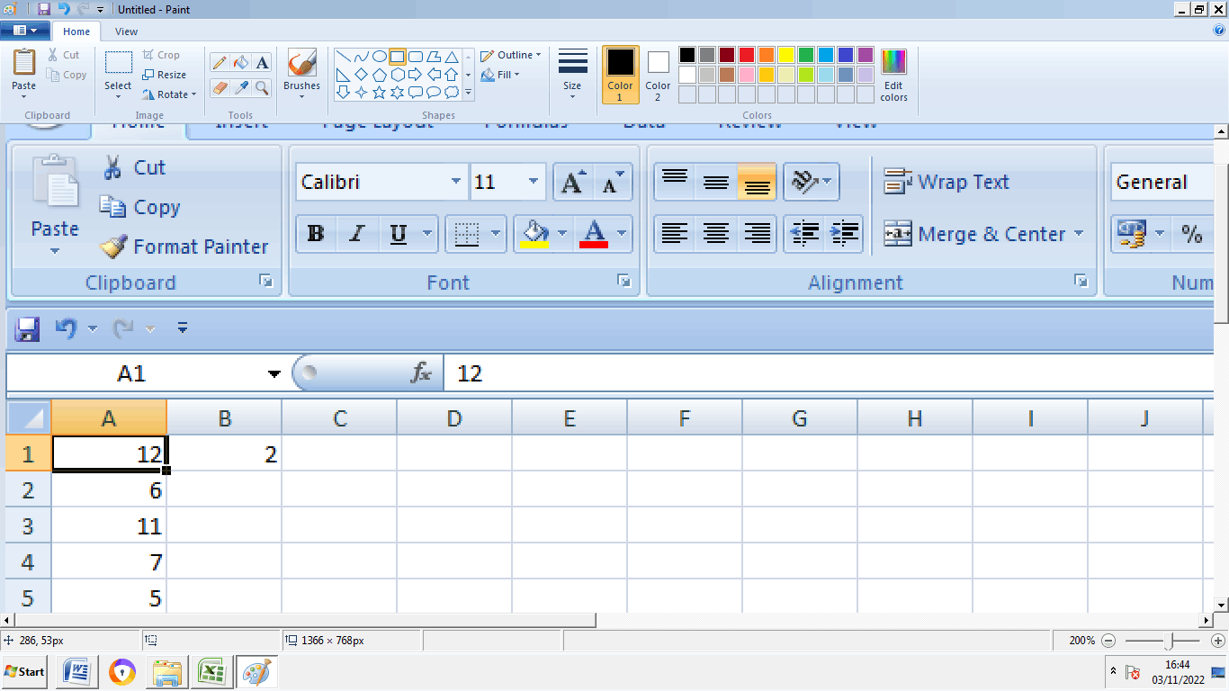
Step 3: Select the cell value B1 and right click. Select the option Copy or use a shortcut method CTRL+C.

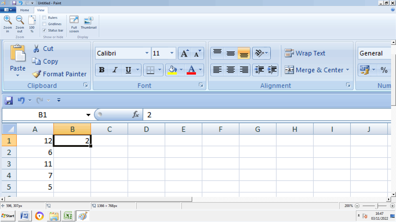
Step 4: Select the range A1:A5.

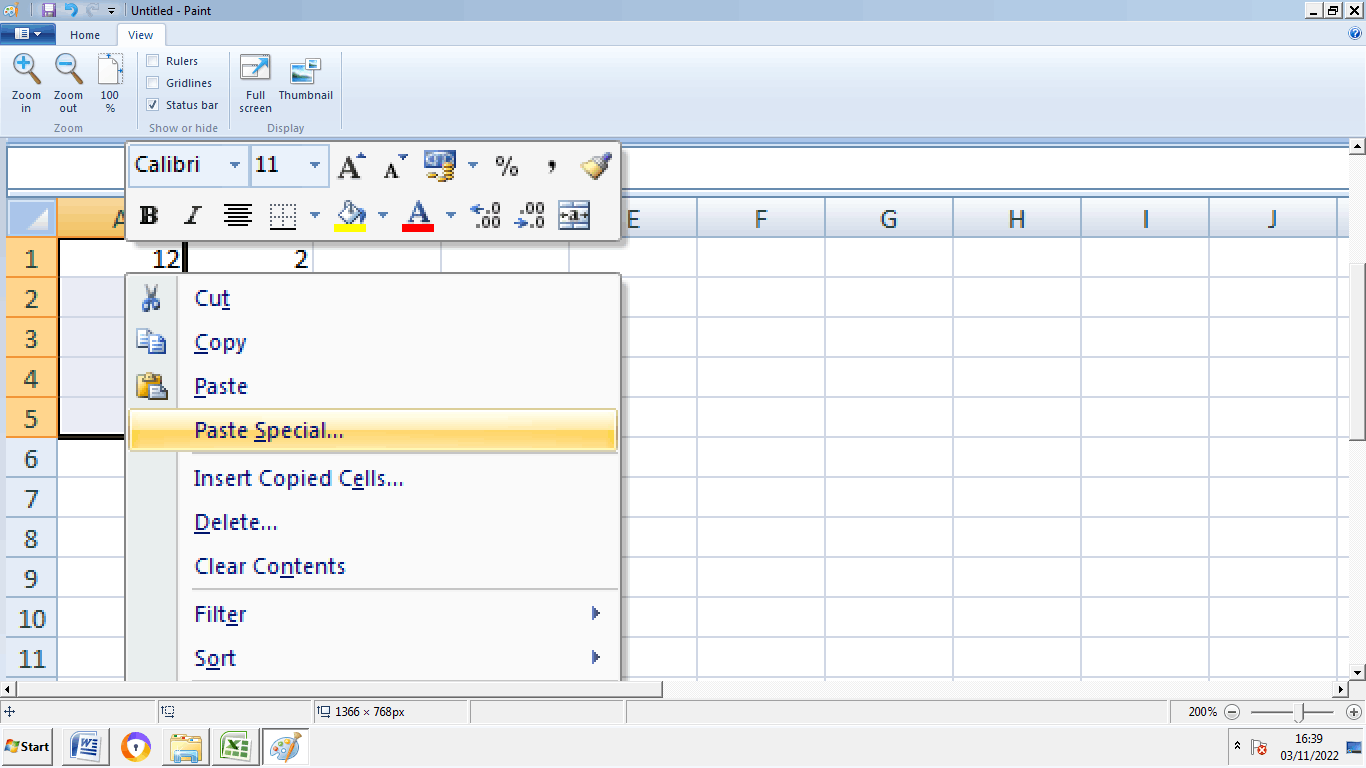
Step 5: Right click towards it and choose the option Paste Special.

Step 6: Click Divide

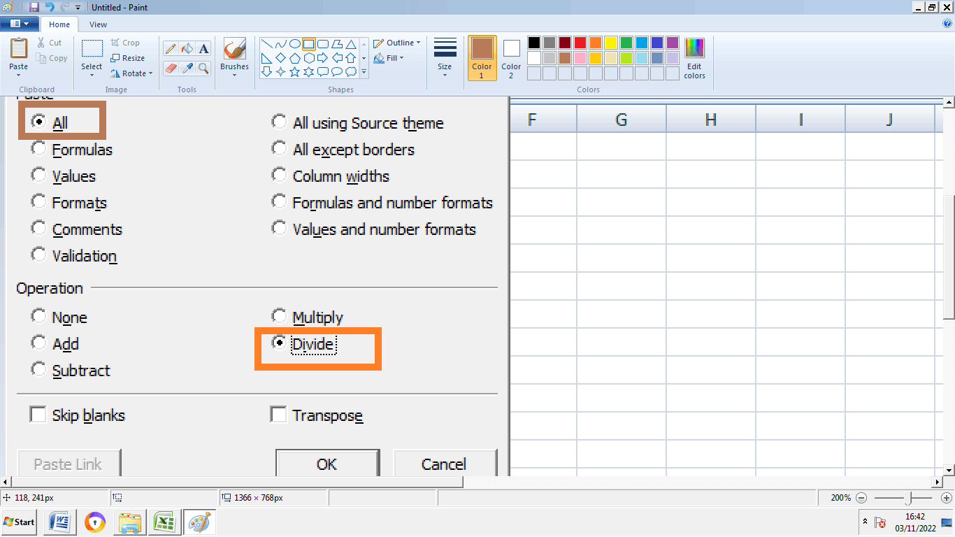
Step 7: Click OK.

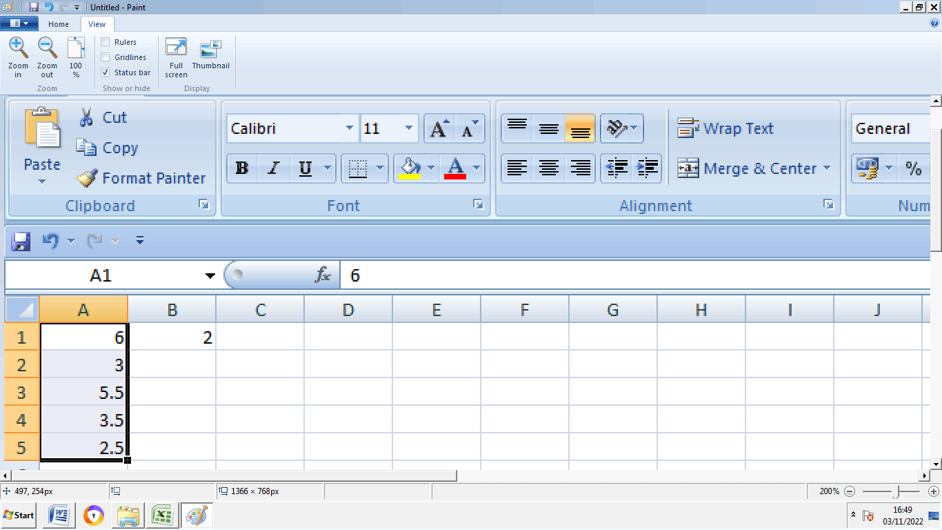
From the above worksheet, the value present in the column range A1 is the result which is divided by the number or value present in the cell B2 .

Summary

From the above tutorial, the various functions and method to divide the number is explained briefly.