Formatting in Excel

Formatting in Excel

Formatting in Excel is used to alter and change the appearance of your data in a standardized form. It also helps you to give a professional look to your reports, worksheets, and workbooks. There are many numbers of formatting options available in Excel. You can choose the required formatting as per your needs. 

Formatting Categories

The options available in Custom Formatting are as follows:

1. Number Formatting
2. Accounting Formatting
3. Currency Formatting
4. Date Formatting
5. Time Formatting
6. Percentage Formatting
7. Fraction Formatting
8. Special Formatting
9. Text Formatting
10. Custom Formatting

Number Formatting

The Number Formatting feature allows us to change or control the appearance of any number without changing the actual value.

Shortcut for Windows

Use CTRL+1 keyboard shortcut to access the Format Cell on Window platform

Shortcut for Mac

Use ?+1 keyboard shortcut to access the Format Cell on Mac platform

Steps to Format a Number

1. Select the cells that you wish to format.

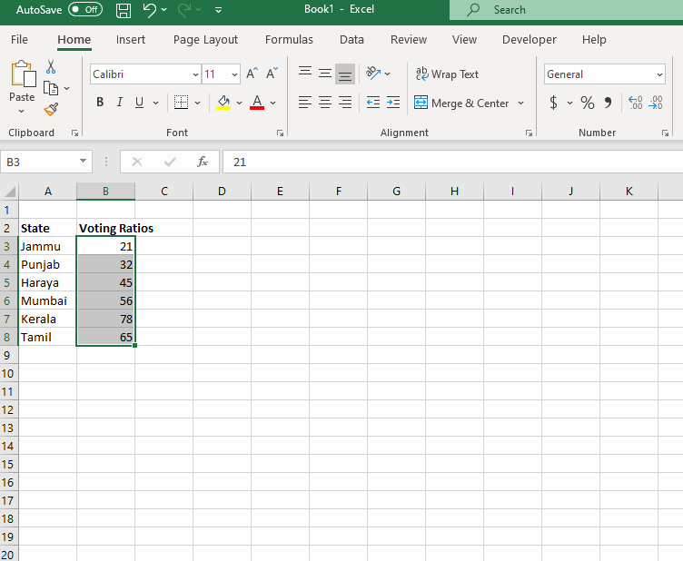
• Click on Home-> Number-> General

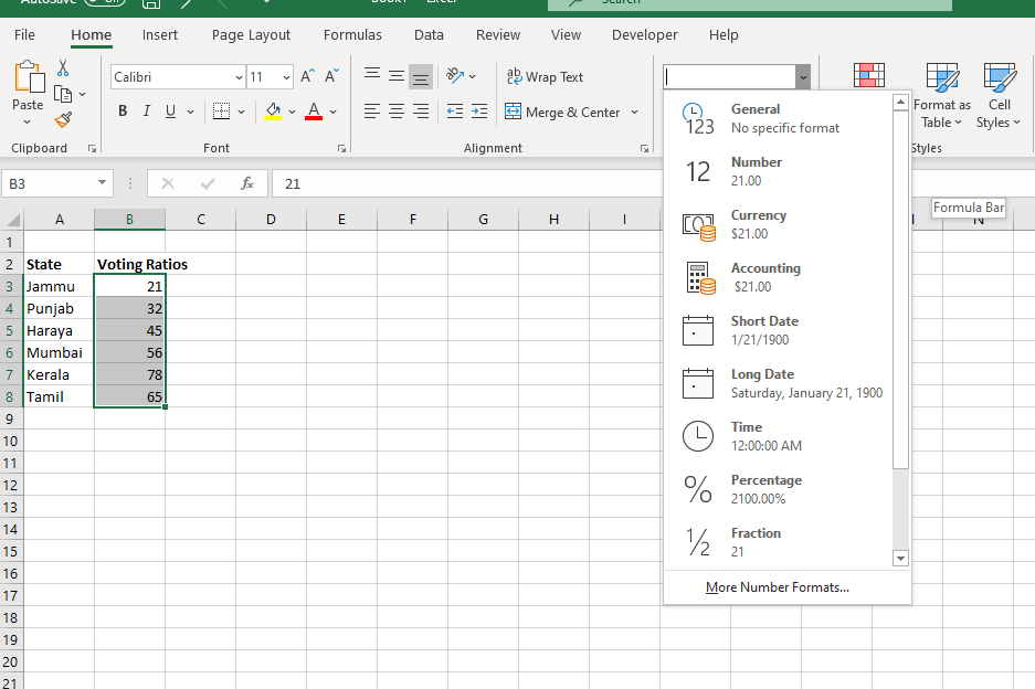
• Various formatting option appears. Choose your formatting category. Here we have clicked on Number formatting. Click on OK

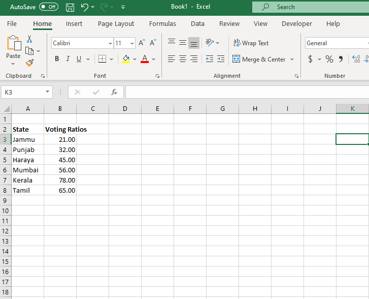
• You will notice that the values have formatted with two decimal digits.

Accounting Formatting

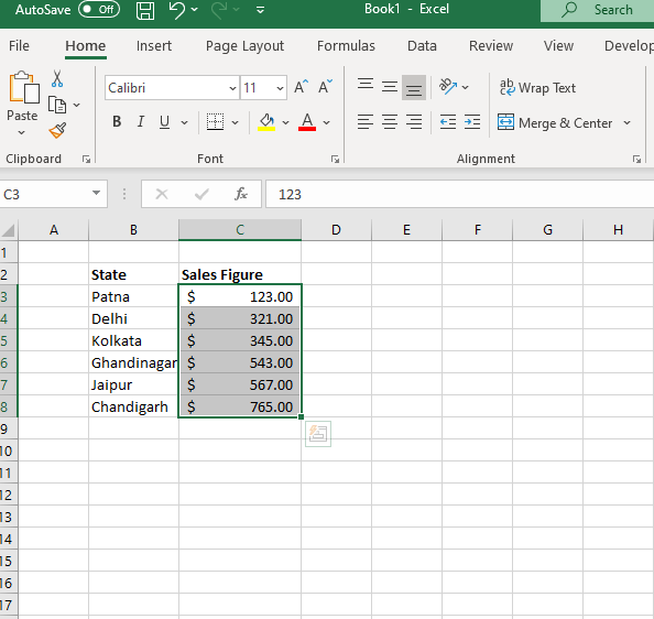
The Accounting format aligns the dollar signs at the left edge of the cell and displays a dash for zero values. It displays negative numbers in parentheses.

Shortcut for Windows

Unfortunately, there is no shortcut, but there are some alternatives. One way is: Alt, H, A, N, Enter.

Shortcut for Mac

None

Steps to Format a Number

1. Select the cells that you wish to format.

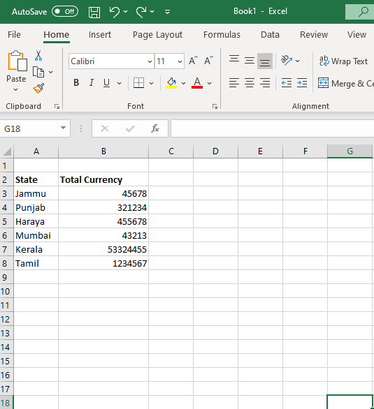
• Click on Home -> Number-> General. A dialog box appears. Either click directly on accounting or click on More Number Formats.

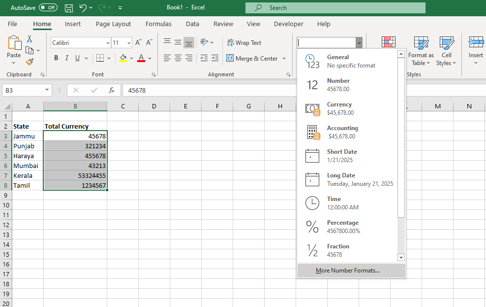
• All the formats will appear. Select the Accounting format. Again, a dialog box will appear.

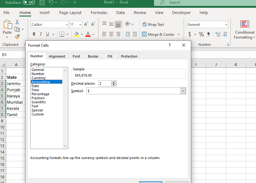
• From symbol choose the currency values, i.e., Indian, euro, dollar, Russian, bitcoin, etc., (default is $) and decimal places for zeros (default value is 2). Click on Ok. You will get the following amount with currency symbols and zeroes.

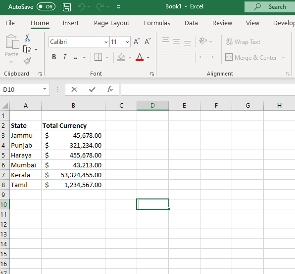
Currency Formatting

Currency formatting is used to assign various currency symbols to your numbers. It is the same as Accounting Formatting but, currency format can display negative numbers with a minus sign, in red, with parentheses, or in red with parentheses.

Shortcut for Windows

Use Ctrl+Shift+$ keyboard shortcut to access the Accounting Format Cell on Window platform

Shortcut for Mac

? + ? + $

Steps to Format a Currency

1. Select the cells that you wish to apply to the currency format.

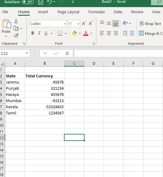
• Click on Home -> Number-> General. A dialog box appears. Either click directly on Currency or click on More Number Formats. A dialog box will appear as given below.

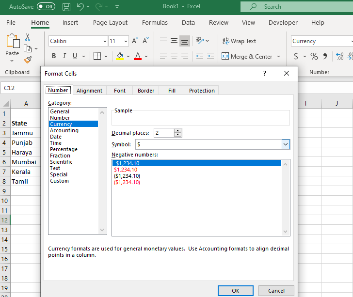
• Choose the currency symbol as per your needs, and you can also assign the formatting for negative numbers. Click on Ok.

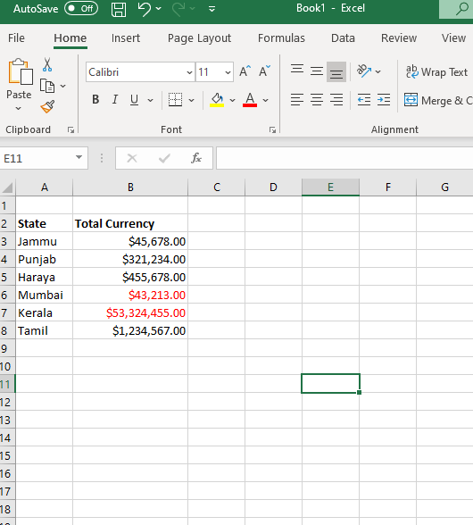
• You will notice all the negative values have turned red.

Date Formatting

Dates are important data in any Project. Date Formatting is used to align the dates systematically such that the further users can understand it, which sharing or reviewing the sheets. Dates can be displayed in different ways using the following 2 options, Short Date, Long Date.

Character	Formatted
D	This character displays the day as a number without a leading zero.
Dd	It is used to display the day as a number with a leading zero when appropriate.
Ddd	It is used to display the day as an abbreviation from Sun to Sat.
Dddd	This character displays the day as a full name from Sunday to Saturday.
M	It displays the month as a number without a leading zero
Mm	This character displays the month as a number with a leading zero when appropriate.
Mmm	This character displays the month as an abbreviation from Jan to Dec.
Mmmm	It displays the month as a full name from January to December.
Mmmmm	This character displays the month as a single letter from J to D.
Yy	It displays the year as a two-digit number.
Yyyy	This character displays the year as a four-digit number

Shortcut for Windows

Use CTRL + SHIFT + #

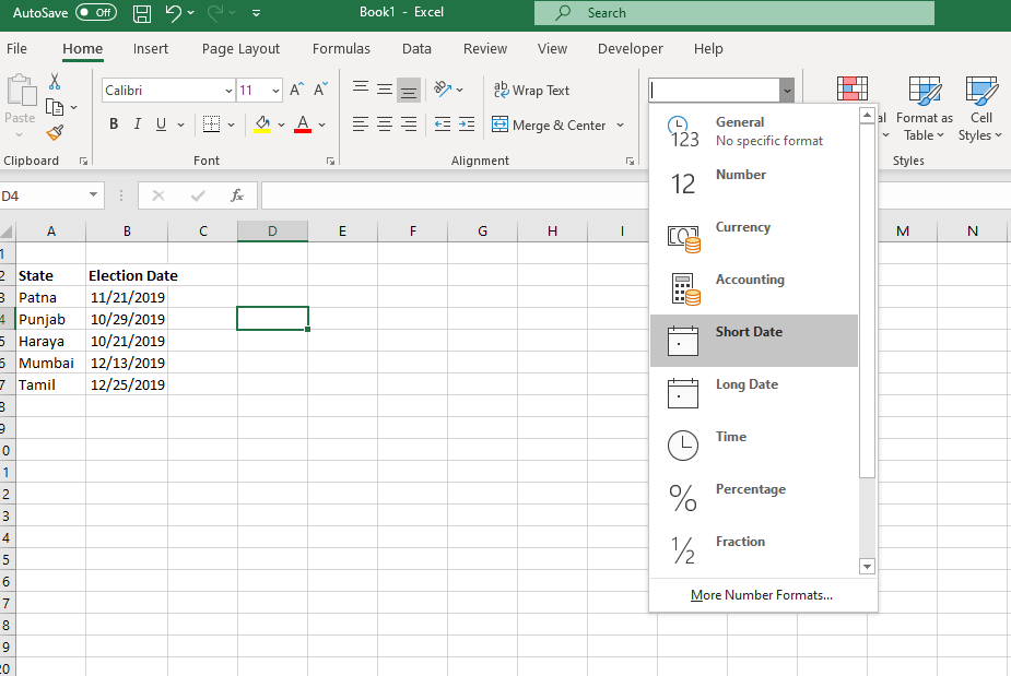
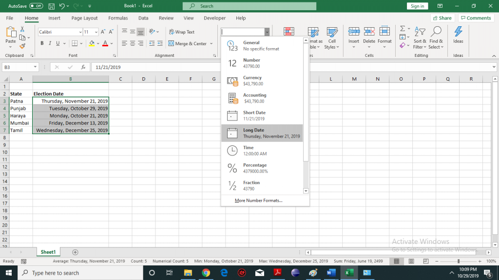
1. Short Date

Select the cells that you want to format. Under Home -> Number->General->Short Date. The format will be mm/dd/yyyy.

• Long Date

Long represents the date in a more detailed manner. Select the cells that you want to format. Under Home -> Number->General->Long. Date. The format will be Day, Month Date, Year.

• Custom Date Formatting

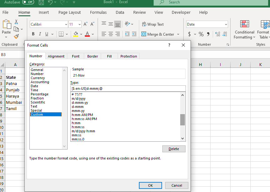
You can create or customized data formatting with the help of Custom Formatting.

Under Home-> Number-> General-> Custom. Either create your own customized date format or choose from the given format.

Shortcut for Windows

Use Ctrl+ 1

Time Formatting

Time formatting assigns the time format in a standardized form.

Character	Explanation
H	This character displays the hour as a number without any leading zero.
[h]	It displays the elapsed time in hours.
Hh	It displays the hour as a number with a leading zero. If the format contains AM or PM, the hour is based on the 12-hour clock else it will be based on the 24-hour clock.
M	This character displays the minute as a number without a leading zero.
[m]	It displays the elapsed time in minutes.
Mm	It represents the minute as a number with a leading zero.
S	This character the second as a number without a leading zero.
[s]	It displays elapsed time in seconds. It returns the number of seconds exceeds 60 if you are working with a formula.
Ss	This character displays the second as a number with a leading zero.
AM/PM, am/pm, A/P, a/p	It displays the hour using a 12-hour clock. Excel displays AM, am, A, or a for times from midnight until noon and PM, pm, P, or p for times from noon until midnight.

Shortcut for Windows

Use CTRL + SHIFT + @

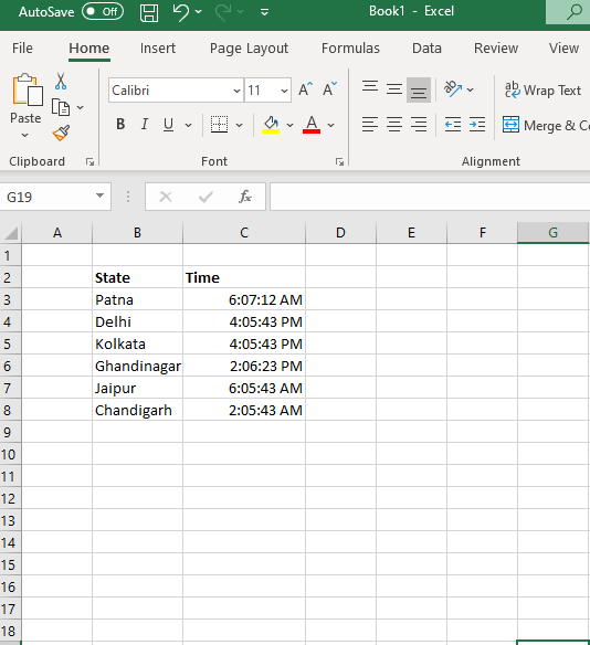
Steps for Time Formatting

1. Select the cells which you want to format.

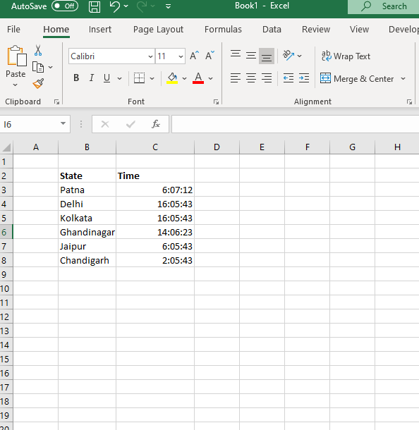
• Click on Home-> Number-> General-> More Number Formats. A dialog box appears.

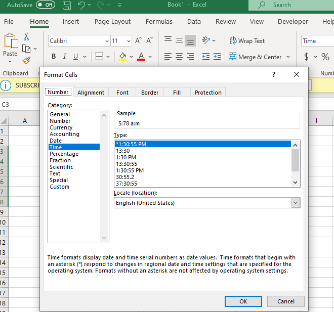
• Select the time format as per your requirement. Click on Ok. You will notice that your time has been formatted.

Percentage Formatting

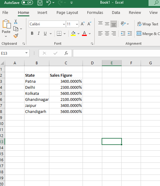
Percentage Formatting formats as a percent. If the percentage format is applied to the cells, then Excel multiplies the number of the cells by 100 to convert it to percentages and displays a dash for zero values. For example, if a cell contains the value 20, after applying the formula 100 will be multiplied to it, the output will be 2000.00 %.

Shortcut of Windows

CTRL + SHIFT + %

Steps for Percentage Formatting:

1. Select the number of cells that you want to format.

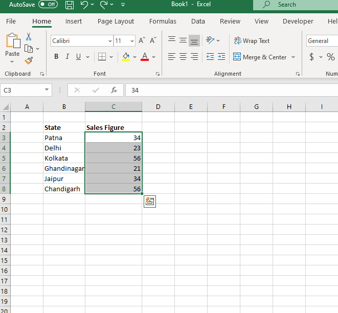
• Under Home, click ->Number->General-> Percentage. The cells will be automatically formatted with percentages.

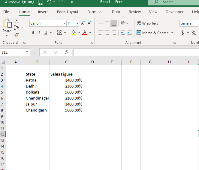
• You can adjust the dash of zeros. By clicking on ‘more number formats’. A dialog box appears. Click on Percentage.

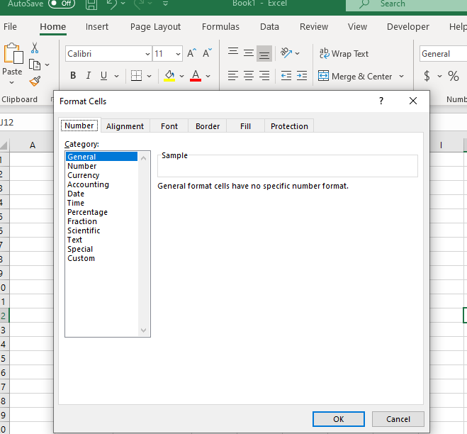
• Click on Percentage. You can choose the decimal places as per your requirement.

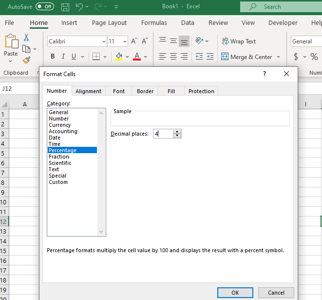
• Click on Ok. Your cell numbers will be formatted with a  dash of four zeros.

Fraction Formatting

Fraction format is used to display or type numbers as actual fractions rather represent them in decimals.

Steps for Fraction Formatting

1. Select the number of cells that you want to format.

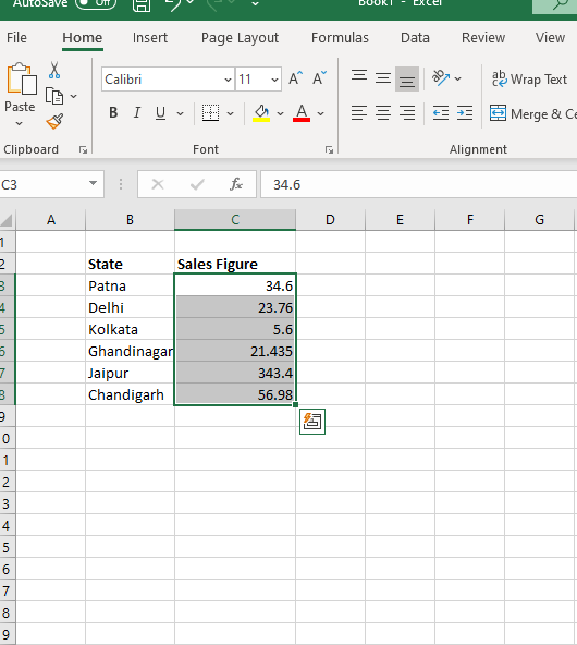
• Click on Home-> Number-> General-> Fractions. The decimal values will be formatted to fractions.

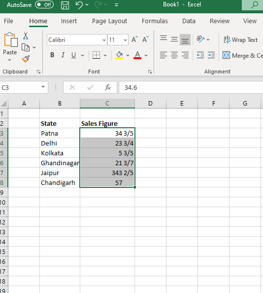
• You can also choose the type of fractions, unlike you want up to one digit, two digits, three digits, halves, quarters, etc.

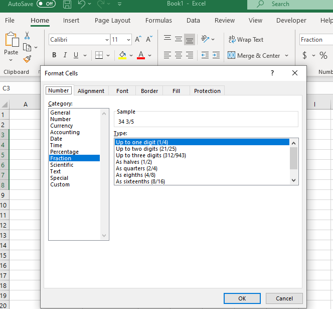
• Choose the desired type and click on Ok. The value will be formatted accordingly.

Special Formatting

Special Formatting is a well- number format category that contains four formats: Zip Code, Zip Code + 4, Phone Number, and Social Security Number.

• Zip Code: This holds any leading zeros in the value. It is important for zip codes that have no importance in arithmetic computations. Example: 0129.
• Zip Code + 4: This code is used to separate the first five digits from the last four digits automatically with a hyphen and holds any leading zeros. Example: 0324-5855.
• Phone Number: This code is used to enclose the first three digits of the number automatically in parentheses and separates the last four digits from the previous three with a hyphen. Example: (989) 555-1011.
• Social Security Number: It puts hyphens in the value to separate its digits into groups of three, two, and four pairs. Example: 555-00-9999.

Steps for Special Formatting

1. Select the cells that you want to format. On the home, click on Number-> General-> More number formats-> Special. A dialog box appears.

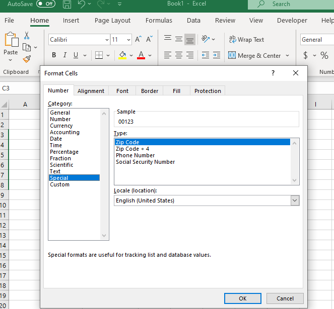
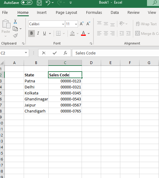
• You will find four different format types, select the desired format as per your requirement (When you select any format type, Excel automatically shows the sample output at the top). Click on Ok. The selected values have been formatted.

Text Formatting

Text formatted cells are treated as text even when there is a number in the cell. The value of the cell is displayed exactly as it was entered. Text formatting is used to embed formatted numbers inside text. It helps to make the output of statistical, financial, or scientific calculations fairer and easier to follow.

Steps to use Text Formatting

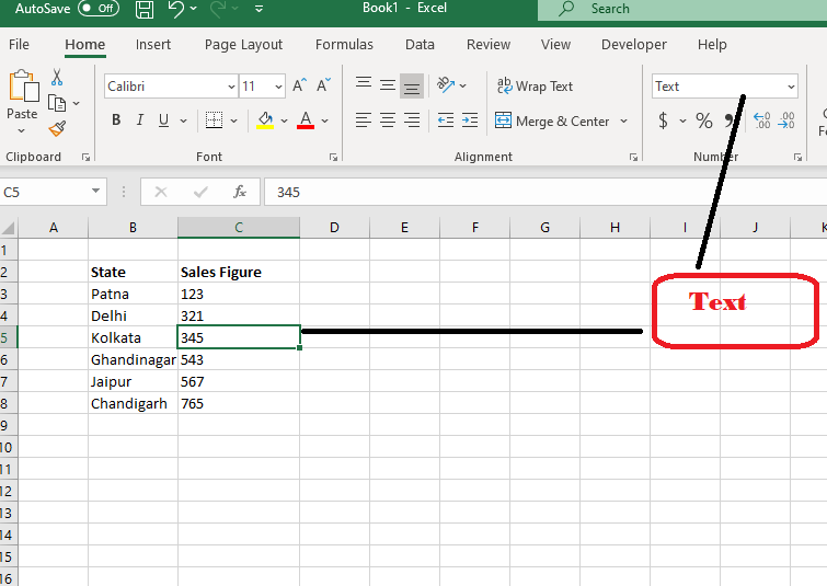
1. Select the cells you at which you want to use text formatting. Click on Home->Number-> General-> more number formats-> text.

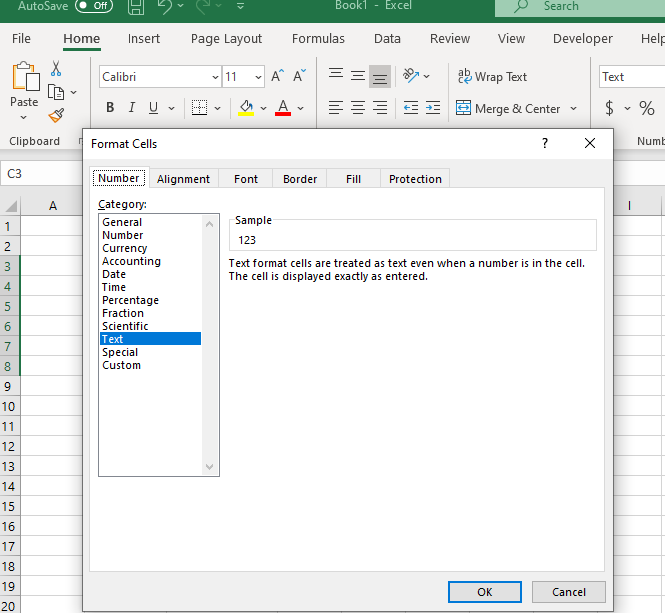
• Click on ok. You will notice that your values in the cells has converted to text.

Custom Formatting

Custom Formatting is used to modify the existing custom code or allows you to enter your own codes from scratch. The Custom category displays a list of codes which one can use for custom number formats, with the help of an input area to enter codes manually in various blends.

Shortcut for Windows

CTRL + 1

Steps to use for Custom formatting

1. Select the cells wherein you wish to apply the custom formatting. Click on Home->Number->General->More number formats-> Custom. A dialog will appear.

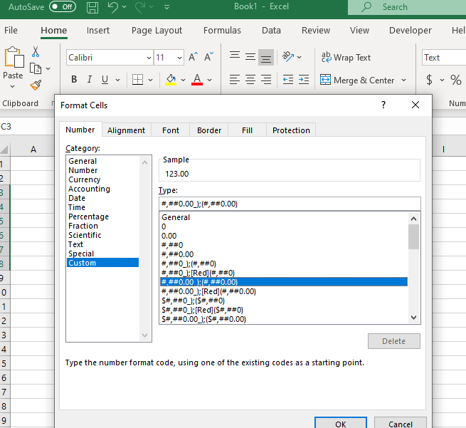
• Enter the code or select from the given code and watch the preview area(sample) to see the result. Click on Ok. You will notice that the selected cells values have been formatted accordingly.