Separate Strings in Excel

How to Separate String in Excel

Day by day, Microsoft Excel is increasing for business and personal use. It is a combination of numbers and alphabets based on the data provided. The data entered by the user is present in different formats. Multiple details are represented in the range of columns. In such data types, the user needs to calculate the specified data present in the range of columns. Hence there is a need to split the particular data from the range of columns.

For example, if the cell contains the person's name and area name, the user must split the area name to finalize the data. In such situations, there is no need to type the data manually in separate columns. One can choose either the formula method or the delimiter character. Formula functions such as RIGHT, LEFT, LEN and FIND can be modified based on the user's preference to split the data. Delimiter includes commas, semi-colons, tabs, and spaces to split the required data from the given data.

But what if someone forgets the formula? There is a method called Flash Fill used to split the data. The formula and flash fill method are clearly explained in this tutorial.

1. How to split the data using the formula method?

The steps to be followed to split the data using the formula method are as follows,

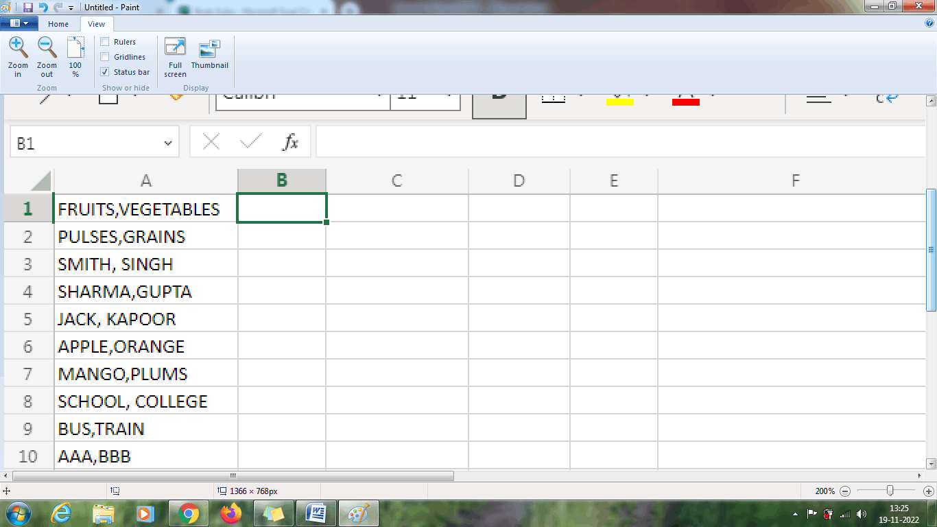
Step 1: Enter the data in the column of range from A1:A10

Step 2: Select cell B1, where the user wants to display the result. Enter the formula in the cell =RIGHT (A2, LEN (A2)-FIND (“,”, A2))

Step 3: Press Enter. The data which needs to be split will display in cell B1. To get the result for the remaining data, drag the formula towards B10.

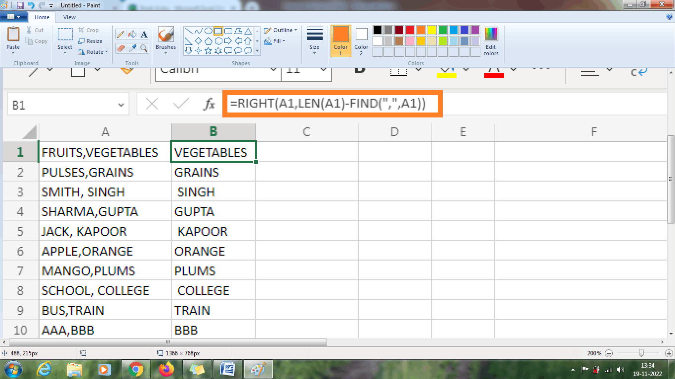
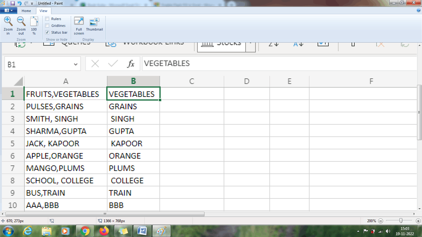
From the above worksheet, using the formula method, the first name is present in another column. From the above formula, the FIND function is used to find the position of the comma, and the LEN function denotes the length of the string. For example, the length of the data present in cell B1 is (17), and the position of the comma is 7. Therefore 17-7=10, where the number 10 indicates the VEGETABLES. Similarly, this method follows all the data in the table.

Example 1: How to split the last name from the data using the formula method?

To split the last name from the data, the steps to be followed are,

Step 1: Enter the data in the column of range from A1:A10

Step 2: Select cell B1, where the user wants to display the result. Enter the formula in the cell =LEFT (A2, FIND (“,”, A2)-1)

Step 3: Press Enter. The data which needs to be split will display in cell B1. To get the result for the remaining data, drag the formula towards B10.

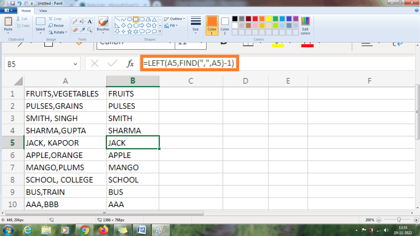
Using the formula method from the above worksheet, the last name is present in another column. Here the formula '-1' indicates removing the comma while displaying the data in the new column.

Flash Fill Method

If one is unfamiliar with the formula method, another method called Flash Fill is used to split the first and last name without the formula method. Here in this example, the steps to display the first name using the Flash Fill Method are as follows,

Step 1: Enter the data in the column of range from A1:A10

Step 2: Select a cell, namely B1, where the user wants to display the result. Enter the first name in cell B1. Here vegetables are entered as the first name in cell B1.

Step 3: Choose File>Options>Advanced options. In that option, check whether the Flash Fill box is checked. Another shortcut method is CTRL+E.

Step 4: Select cell B1. Either one can use the shortcut method or Excel options. The result will be displayed for the rest of the cells, which is the data's first name.

The above worksheet displays the first name in the column range from B1:B10.

 Example 2: How to display the last name using the Flash Fill Method? The steps to be followed are as follows,

Step 1: Enter the data in the column of range from A1:A10

Step 2: Select a cell, namely C1, where the user wants to display the result. Enter the last name in cell B1. Here fruits are entered as the last name in cell B1.

Step 3: Choose File>Options>Advanced options. In that option, check whether the Flash Fill box is checked. Another shortcut method is CTRL+E.

Step 4: Select cell C1. Either one can use the shortcut method or Excel options. The result will be displayed for the rest of the cells, which is the data's last name.

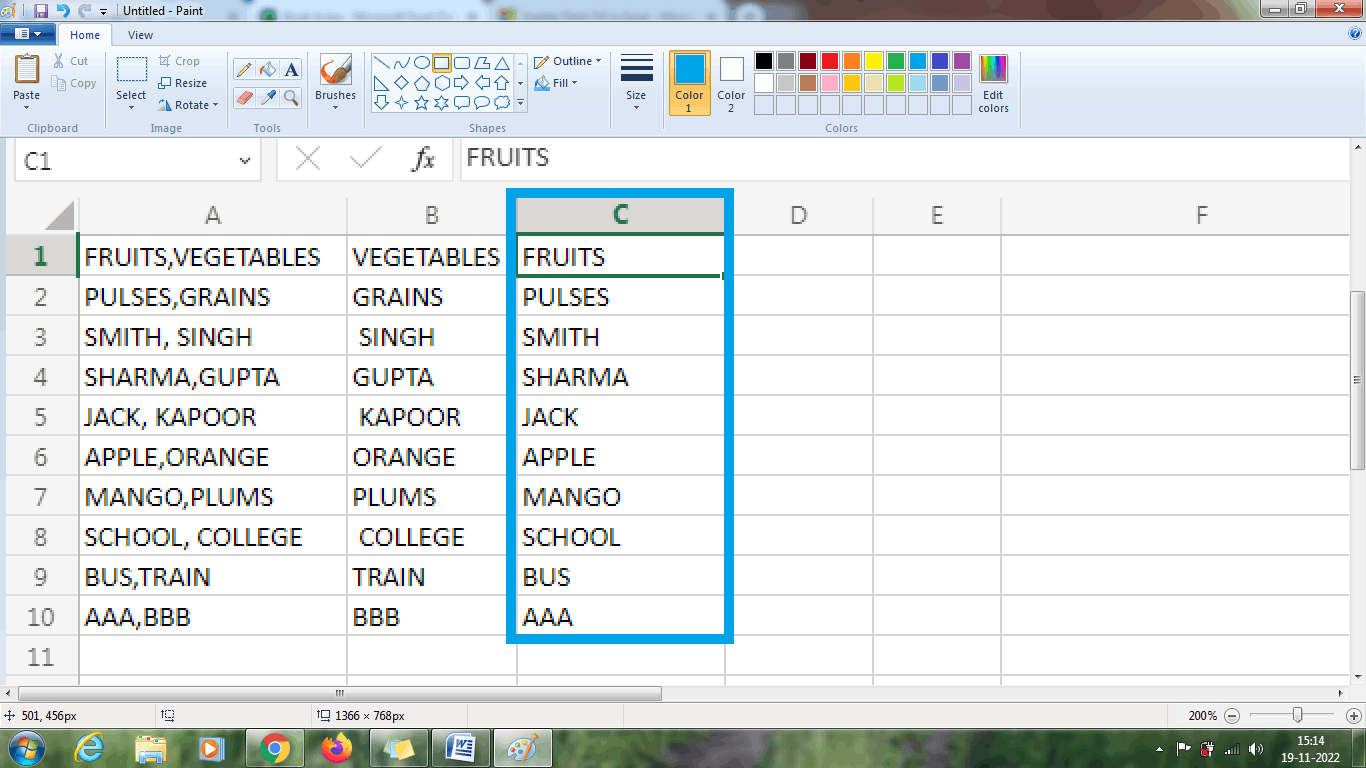
From the above worksheet, the last name is displayed in the column range C1:C10 using Flash Fill Method.

Summary

From the above method, the various functions and methods to separate the strings are explained briefly.