Nearest Multiple in Excel

In Excel, the values in Multiplication can be round up, down and to nearest Multiplication number using Excel default function. This makes the calculation to be performed in an easier and quicker way. Excel provides default function like FLOOR, CEILING and MROUND to round off the nearest multiple in Excel.

1. How to round a number down or nearest multiple using Excel default function?

To round a number to its nearest multiple, the function used is MROUND and FLOOR. Here FLOOR function is used to round a number down to the nearest multiple values.

The syntax of the formula is,

=FLOOR (number, multiple)

=MROUND (number, multiple)

The steps to be followed are,

Step 1: Enter the data in the cell namely A1.

Step 2: Select a new cell, where the user wants to display the result namely B1.

Step 3: Enter the formula in the cell as =MROUND (A1, 5). Here the number is rounded to nearest multiple of 5.

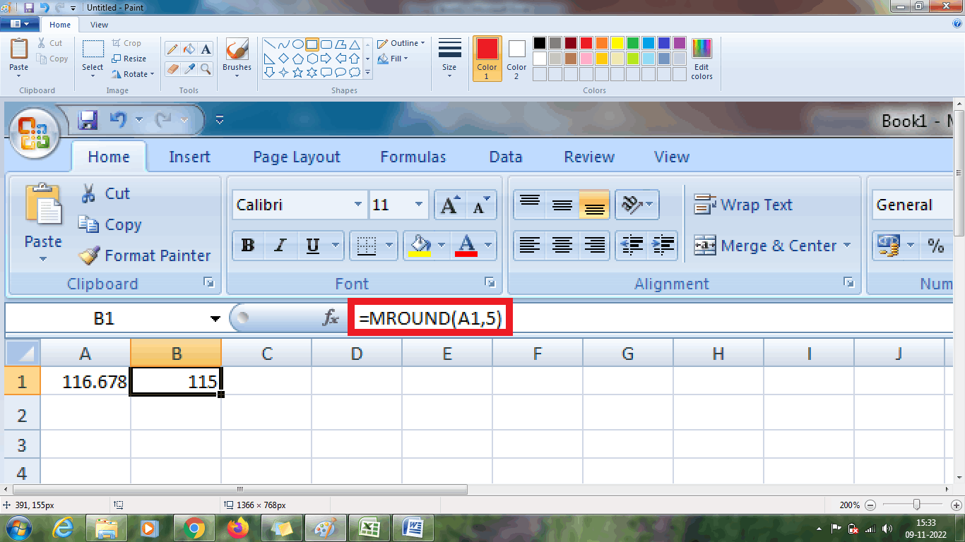
From the above worksheet, using MROUND function the value is rounded near to the multiple of 5. Similarly FLOOR function is used to rounding a number down to the nearest multiple. To use this function, the steps to be followed are,

Step 1: Enter the data in the cell namely A1.

Step 2: Select a new cell, where the user wants to display the result namely B1.

Step 3: Enter the formula in the cell as =FLOOR (A1, 6). Here the number is rounded to nearest multiple of 6.

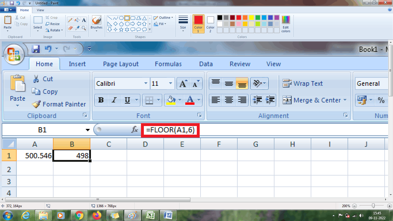
From the above worksheet, the FLOOR function is used to round down to the nearest multiple of 6.

Here is an another example, to round down to the nearest multiple of 2. The steps to be followed are,

Step 1: Enter the data in the cell namely A1.

Step 2: Select a new cell, where the user wants to display the result namely B1.

Step 3: Enter the formula in the cell as =FLOOR (A1, 2). Here the number is rounded to the multiple of 2.

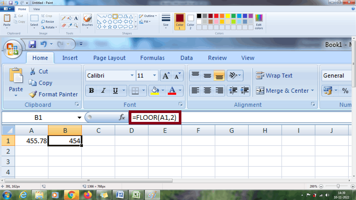
From the above worksheet, the FLOOR function is used to round down to the nearest multiple of 2.

2. How to round up a number in multiple using Excel default function?

To round up a number to its nearest multiple, the function used is CEILING. The steps to be followed are,

Step 1: Enter the data in the cell namely A1.

Step 2: Select a new cell, where the user wants to display the result namely B1.

Step 3: Enter the formula in the cell as =CEILING (A1, 10). Here the number is rounded up to nearest multiple of 10.

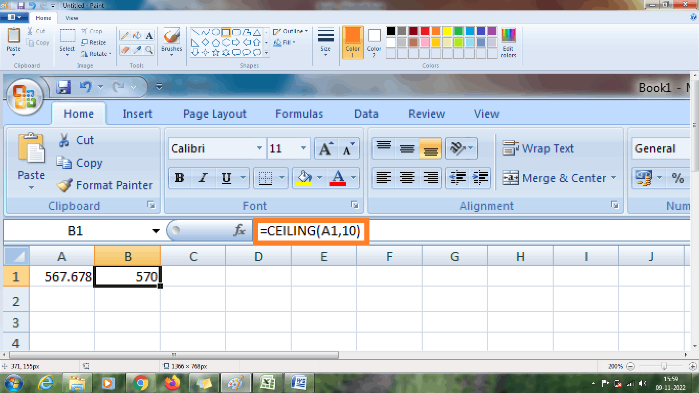
From the above worksheet, using CEILING function the value is rounded up near to the multiple of 10.

Here is an example, to round the value up to the nearest multiple. The steps to be followed to round the values near to the multiple of 7 is,

Step 1: Enter the data in the cell namely A1.

Step 2: Select a new cell, where the user wants to display the result namely B1.

Step 3: Enter the formula in the cell as =CEILING (A1, 7). Here the number is rounded up to nearest multiple of 7.

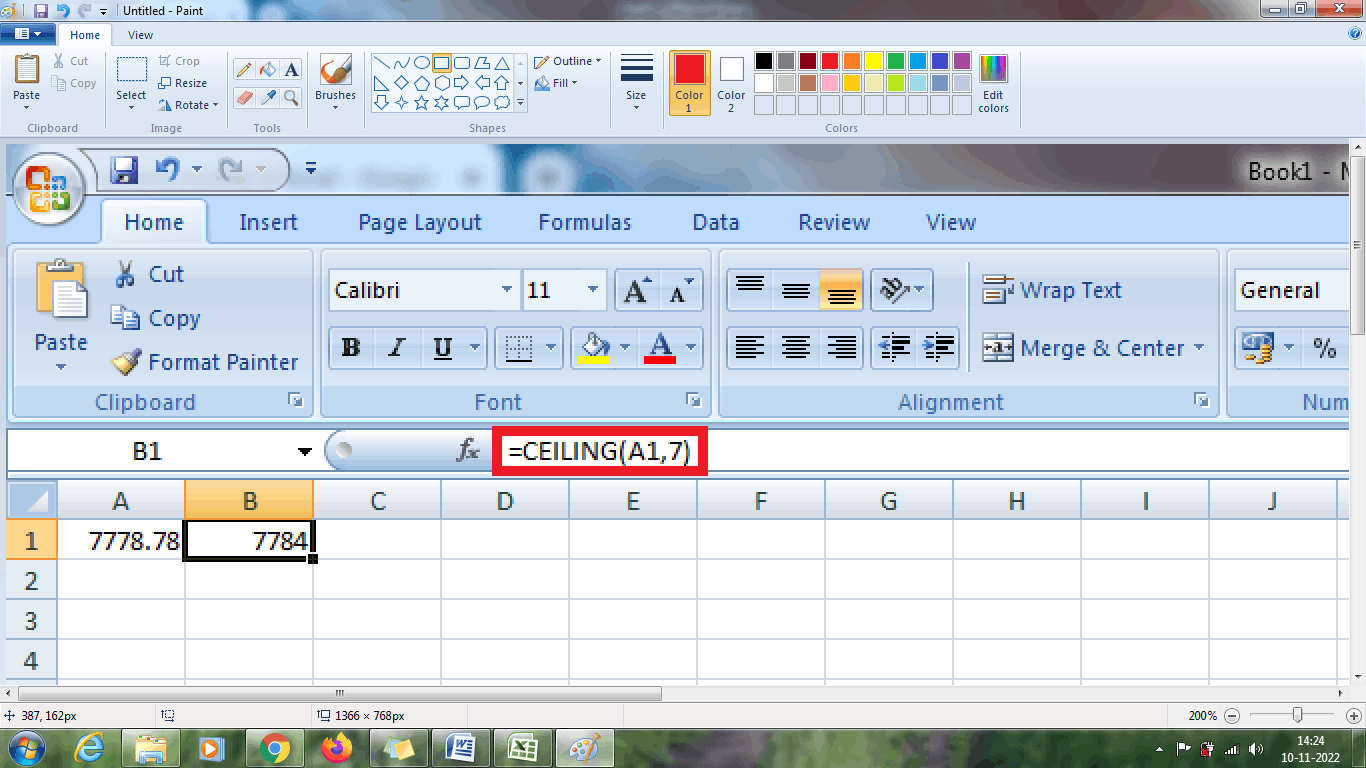
From the above worksheet, using CEILING function the value is rounded up near to the multiple of 7.

Summary

From the above tutorial, the various functions and methods to round the value to the nearest decimal is clearly explained.