Dependent Drop-down List in Excel

Excel forms are used to fetch data from the end user. When we have to give choices, we often use the drop-down feature of Excel. In this tutorial, we won’t be discussing drop-downs. Instead, we will cover the dependent drop-down list.

What is a dependent drop-down list?

 In Excel, if more than one drop-down list is needed, the items in the second list can vary depending on the value of the first drop-down list. This process is called a Dependent Drop-Down list. The other names of the drop-down list are DDL or drop-down menu, pull-down list, or pick list.

Features of Drop-down List

The features of the drop-down list are listed below.

• Items- The user includes items in the list, which contains various things one can select according to their choice.
• Value- The user selects the item currently called value.
• Style – Style is an option in a spreadsheet that includes various properties like color, font size, weight, etc.
• Alignment – Alignment is allowed to choose the position of the item within the button.
• Elevation- This feature is to elevate the dropdown list or menu.
• Icon – It is used to display the icon in the dropdown list
• Icon Size- This feature determines the size of the hero.
• Icon Disabled Color – When the dropdown button is disabled, the icon color is set
• Icon Enabled Color- The icon color is set when the dropdown button is enabled.
• Dropdown Color – This dropdown property determines the background color of the dropdown.
• Is Dense- The height of the button is reduced using this property
• Is Expanded- This feature enables the dropdown button to full width
• SelectedItemBuilder – The user selects the option from the drop-down list displayed on the button. When the user wants to show another text instead of the selected option SelectedItemBuilder option is used
• Hint – The user can choose their desired text from the list to set as the default option in the list.
• Disable Hint – It displays the desired text of the user when the drop-down button is disabled.

Types of Creating Dropdown List

One can create a drop-down list for various types, such as,

1. Selection – A drop down used to select single items from multiple choices in the form
2. Search Selection – It allows the user to search through many options.
3. Multiple Selection – It allows one to select multiple choices from the option.
4. Multiple Search Selection – A selection dropdown can allow multiple search selection
5. Search Dropdown – A dropdown can be a searchable one.
6. Search in Menu- It includes a search prompt inside a menu.
7. Inline- It is formatted to appear inline in other content
8. Pointing- A dropdown can be formatted so that the menu is pointing

How to create a Dependent drop-down list in Excel?

A dependent drop-down list is used to create data entry forms or Excel Dashboards. The drop-down list is helpful when using us to enter a list of products, regions, etc., where the user often needs to join the cell.

STEP 1: Enter the data set in the spreadsheet

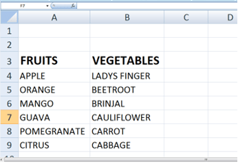
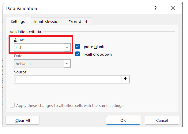
STEP 2: Select the cell where the drop-down list wants to display as C4. Choose data -> data validation. A dialogue box appears. Select the list option from the Allow drop-down and in the source window specify the range of data for which you want to apply the drop-down i.e, A3:B3.

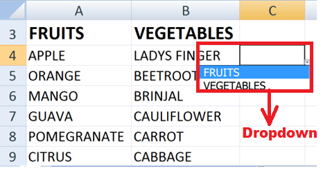
STEP 3: A drop-down list is created for fruits and vegetables is shown below

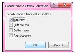
STEP 4: Select the whole data from A3:B9. Choose Formulas, in the Defined Name tab, select Create from Selection. A dialog box appears in that choose “Top Row” and click OK.

STEP 5: Select the cell where you want the conditional/Dependent drop-down list as D4.

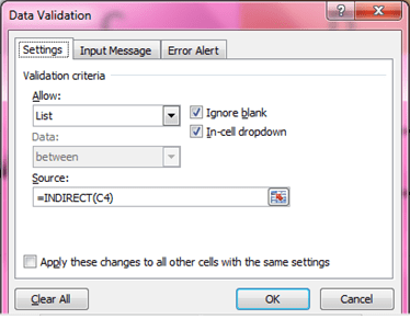
STEP 6: Choose Data> Data Validation and select list from the dialogue box.

STEP 7: In the Source field, enter the formula =INDIRECT (E4), where E4 is the cell which contains the main drop-down list. Then click OK.

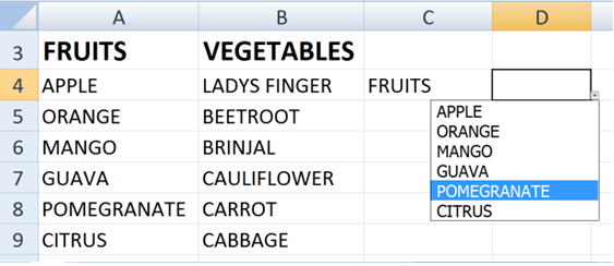
STEP 8: The final result is shown below.

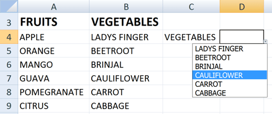
In the above image, the items in the drop-down list D4 are displaying depending upon the drop-down list 1.

After Fruits are selected from the main dependent list C4, the items in the drop-down list D4 vary regarding the value from the main dependent list.

Create a Named Range for a List of Items

The alternate way to enter the list items in the drop-down menu is by entering them in a named range and referencing the prescribed content in the Data Validation Menu.

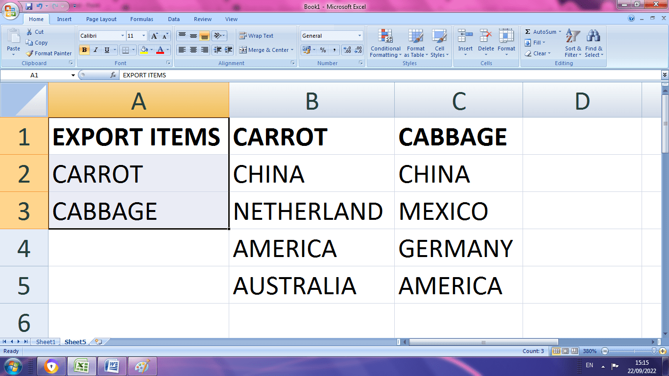
STEP 1: A required data is entered in the spreadsheet

STEP 2: Select the range of cell to create a named range .It should be a single range of column

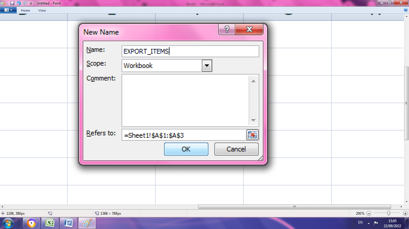
STEP 3: Select the Define Name command from the Formula tab. The New Name dialogue box will appear. Enter the name and range in the box as shown above. Press OK.

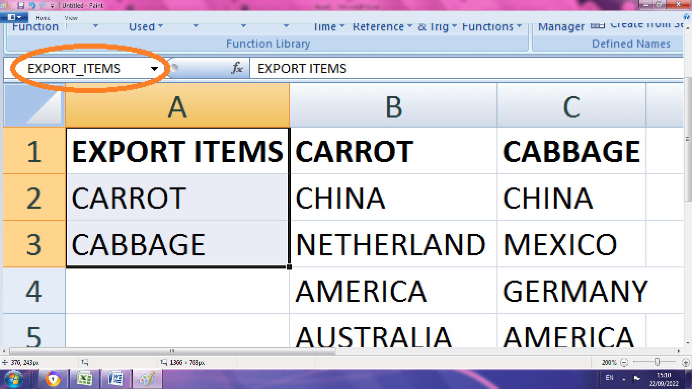
STEP 4: This will create the name; if the range is selected, the term is displayed in the Name Box.

After creating the name range, the user can create their drop drown list.

To create a drop-down list, first, select the cell.

Then choose the data validation option and the List option in the Allow button.

From the Source input box, enter the named range for the list source, which is preceded with an equal sign. Press Enter key.

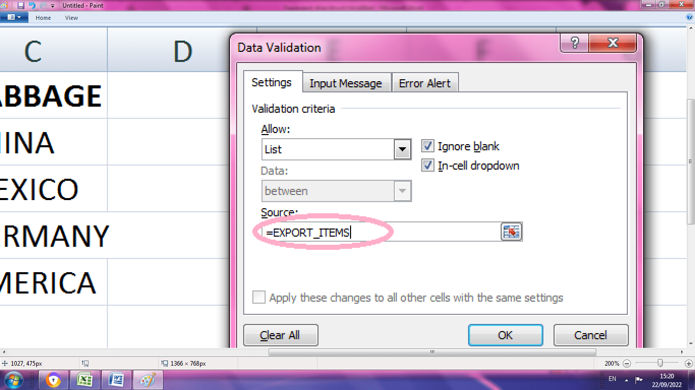
From the above image the source name is displaying automatically when the particular range is selected.

The above image shows the drop-down menu displaying the item of the selected range.

The pros are the user can use this range name as a single source for many data validation lists. The user can edit the named range, which will reflect in the drop-down list that uses the content.

If the range name is moved to another location in the spreadsheet, it acts as a good source for drop-down lists that use it as a source for list items.

The cons are that first need to set the range name, but if many dropdowns in the spreadsheet are using the same source, it acts as an overhead.

Use a Table for List Items

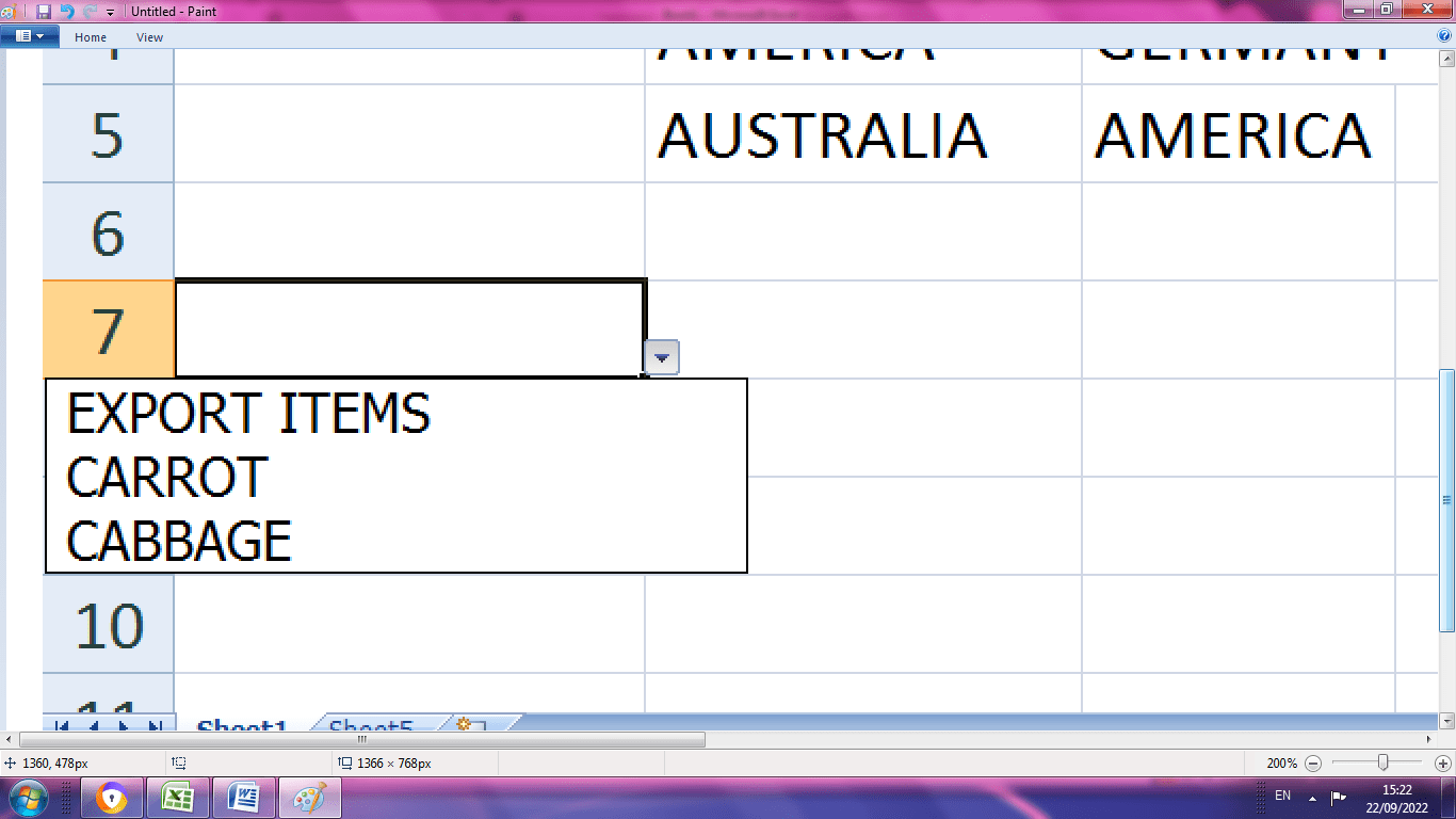
Tables are used to add new data to the table. Typing the latest data below the table will add the new data to the table. The new entries in the table will add to the list below as a list item source.

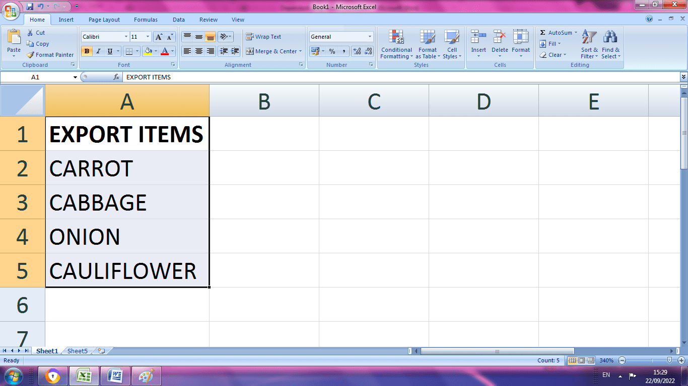
Step 1: Select the data for the table, including the header.

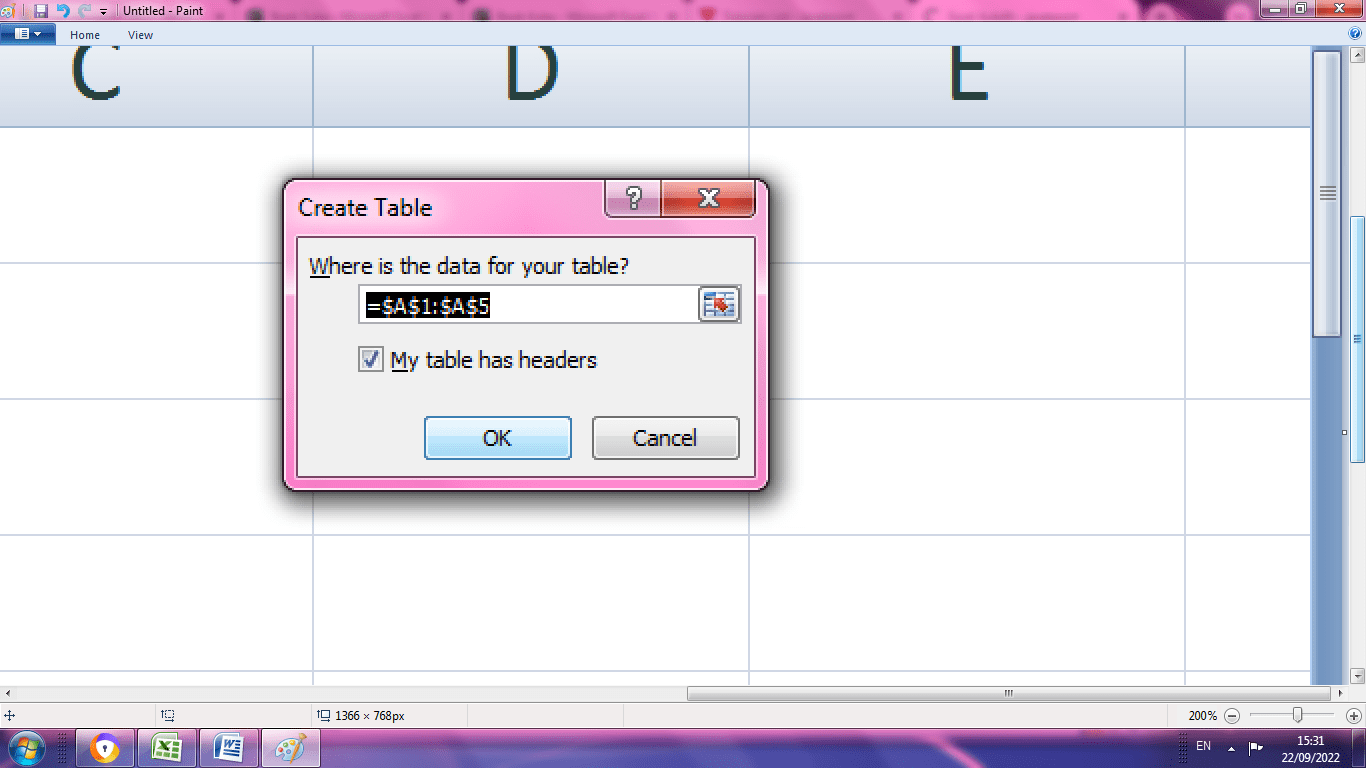
Step 2: Go to Insert Tab and click the Table button in the Tables group of the ribbon.

Step 3: A dialogue box appears, where the range is selected to create the table. Press the OK button after selecting the content. Check whether the header option is checked.

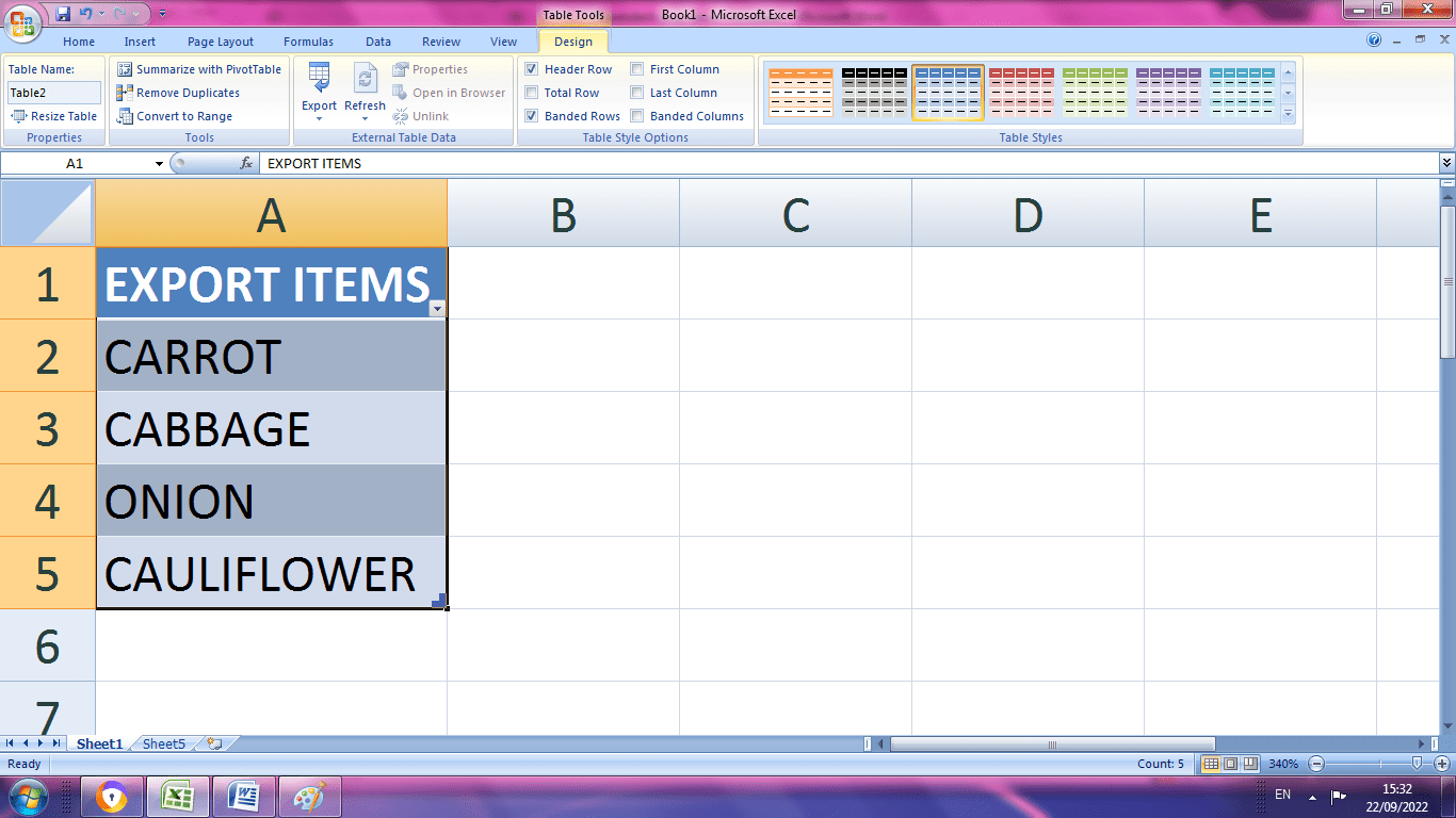
STEP 4: A table is created for the required data as shown below. This table accepts the new data if added.

Multi-Level Dependent Drop-down List

“If more than one dependent drop-down list present, it is called Multi-level Dependent drop down list.”

 One list depends upon one or more main list .The value in the list changes depends upon the value in the other list. For large sets of data Multi-Level Dependent Drop-down list is created.

How to create a Multi-Level Dependent Drop-down List?

To create a Multi Dependent Dropdown List following steps are followed.

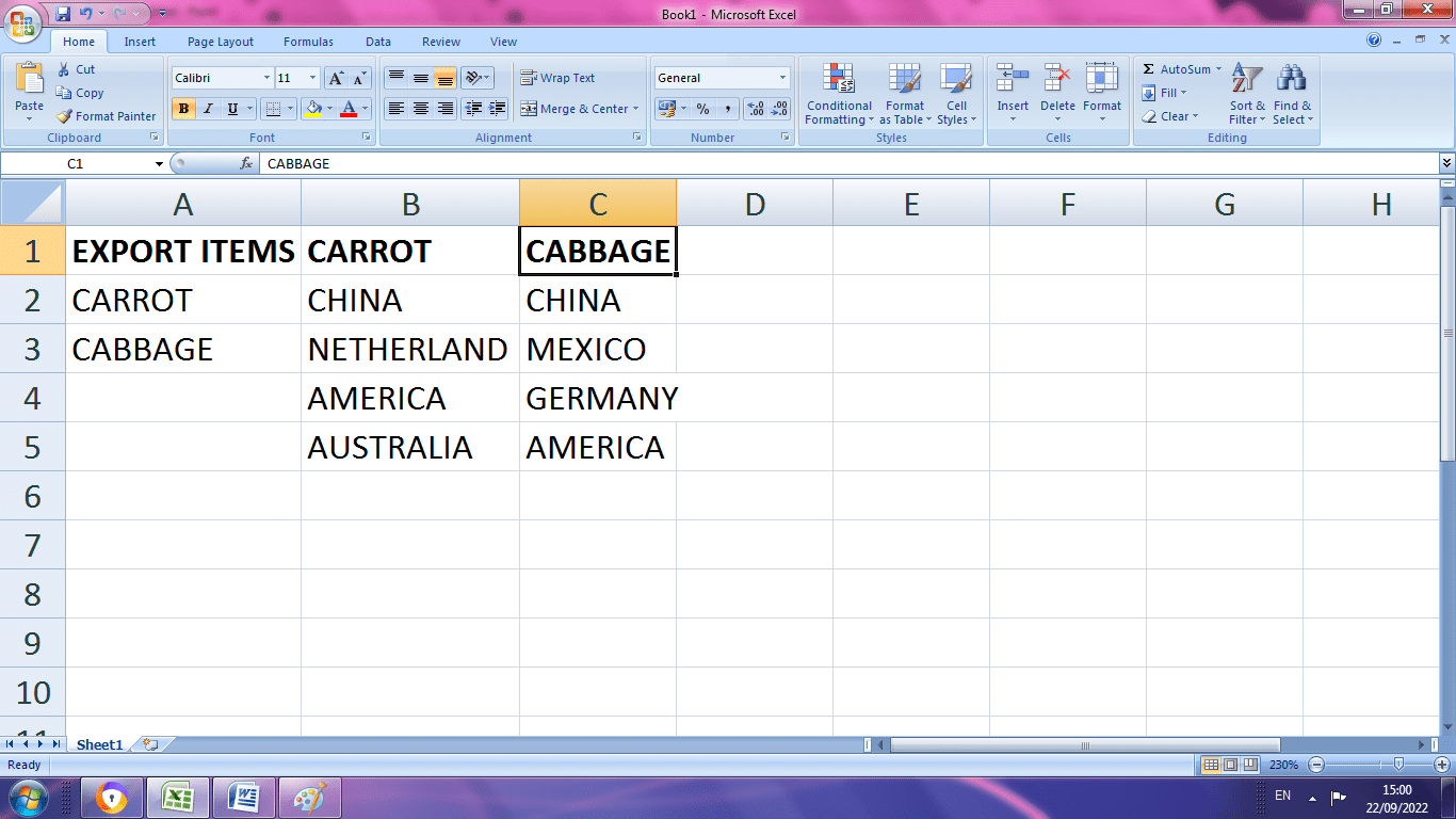
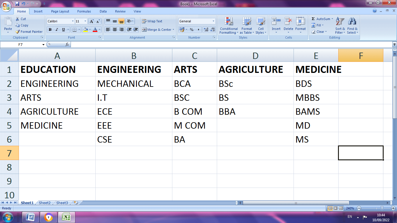
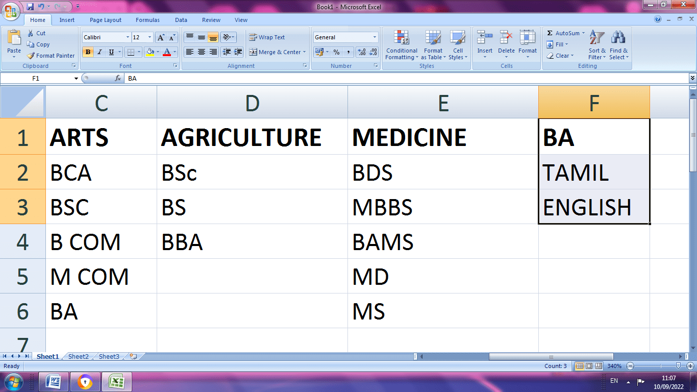
STEP 1: Create the spreadsheet entries that need to appear in the drop-down list. The first column indicates the primary source, while the other three indicate the dependent drop-down list.

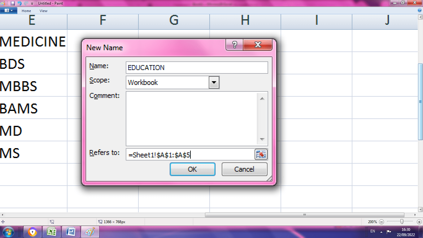
STEP 2: Create a named Range for all entries by selecting Formula bar> Name Manager in Defined Names. A dialog box appears, in that click New. Select the required name and range.

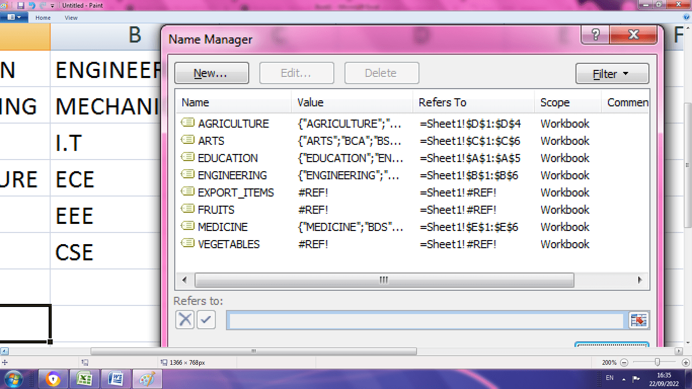
STEP 3: Similarly create the named range for all the fields as shown below.

Step 4: Create the first drop-down list by selecting Data> Data Validation. Choose List and type the source name from named ranges.

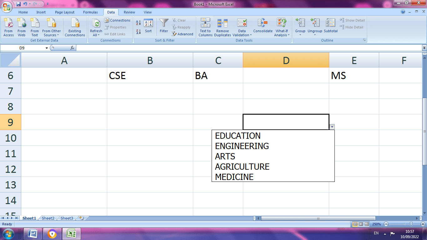
STEP 4: Create a Dependent Drop Down list using the formula =INDIRECT (D9), where D9 is the main list.

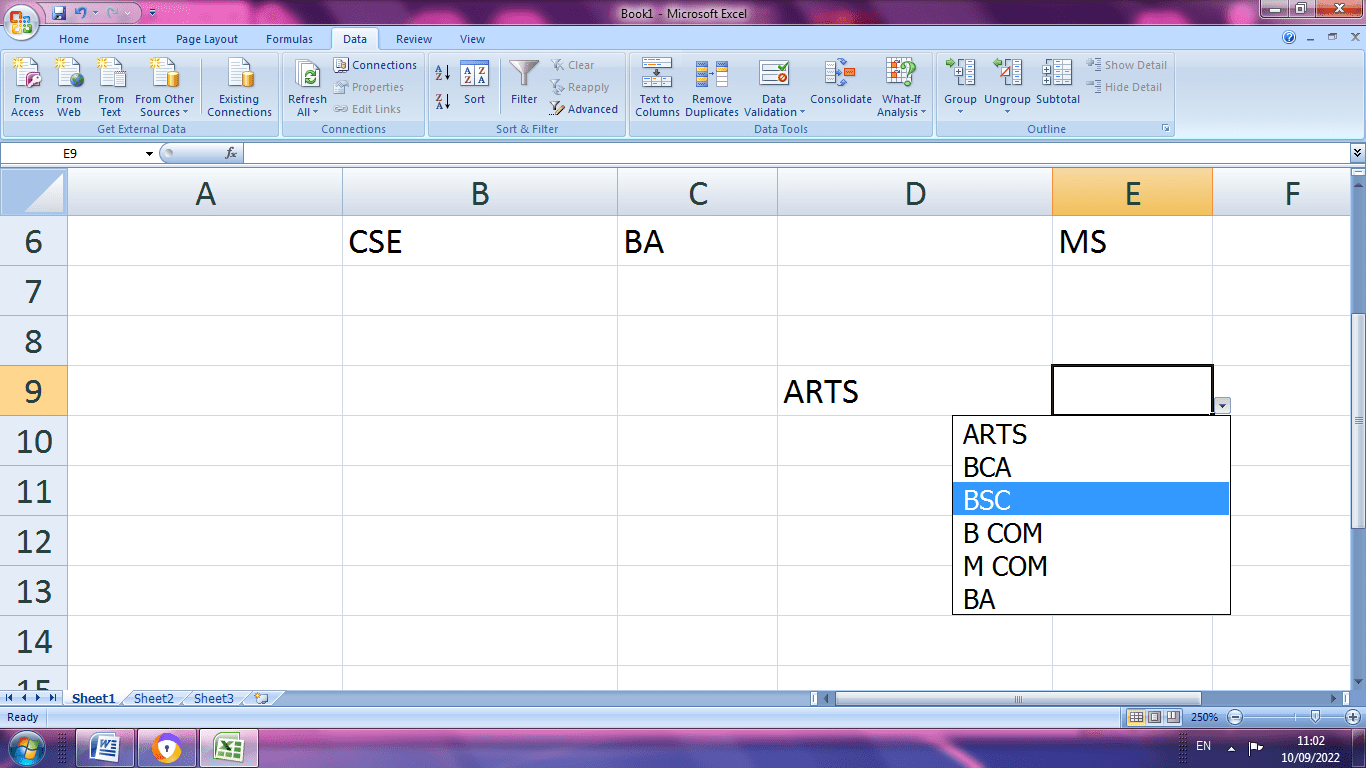
The dependent list varies upon the value in the first range.

STEP 5: To create Multi dependent drop-down list, start a third data as shown below. Under the BA category, Tamil and English are added.

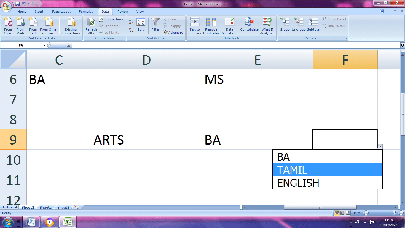
STEP 6: The multi-dependent drop-down list is created from the below images. By choosing under Arts>BA>TAMIL. It is made using the formula =INDIRECT (E9), where E9 is the main list of F9.

How to add color to the dropdown list?

Colour plays a vital role in the Excel drop-down list. Adding color to the drop-down list cells is a more straightforward task, and it is done by adding conditional formatting rules.

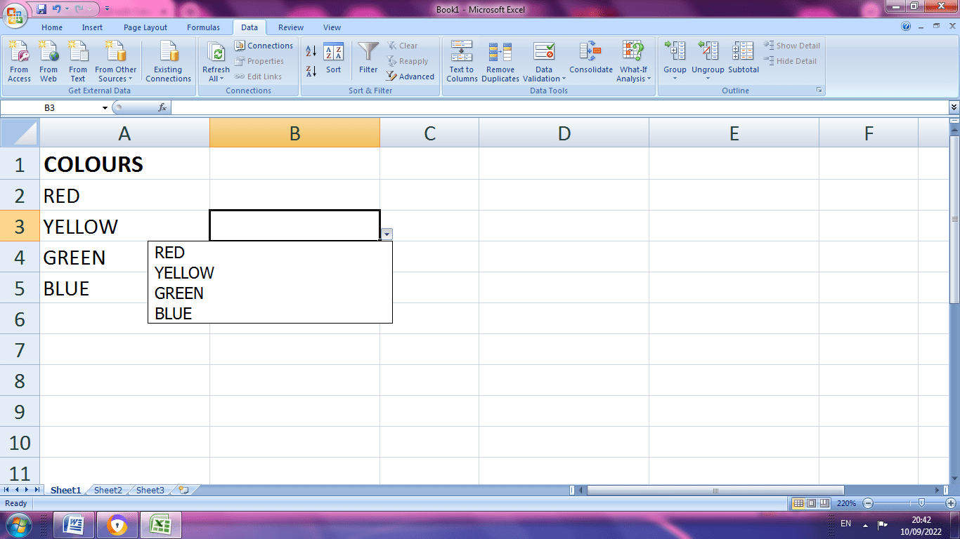
STEP 1: Create data in a spreadsheet, create a dropdown list using data validation, and select the specified range.

STEP 2: A drop-down list is created, as shown in the above image.

STEP 3:  Select the cell where the drop-down list is present. Then choose Home>Styles Group > Conditional Formatting.

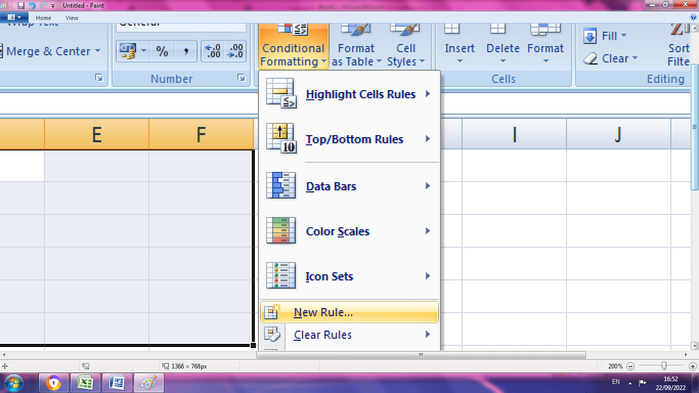
STEP 4: Choose Highlight Cell Rules>More Rules. A format rule dialogue box will appear.

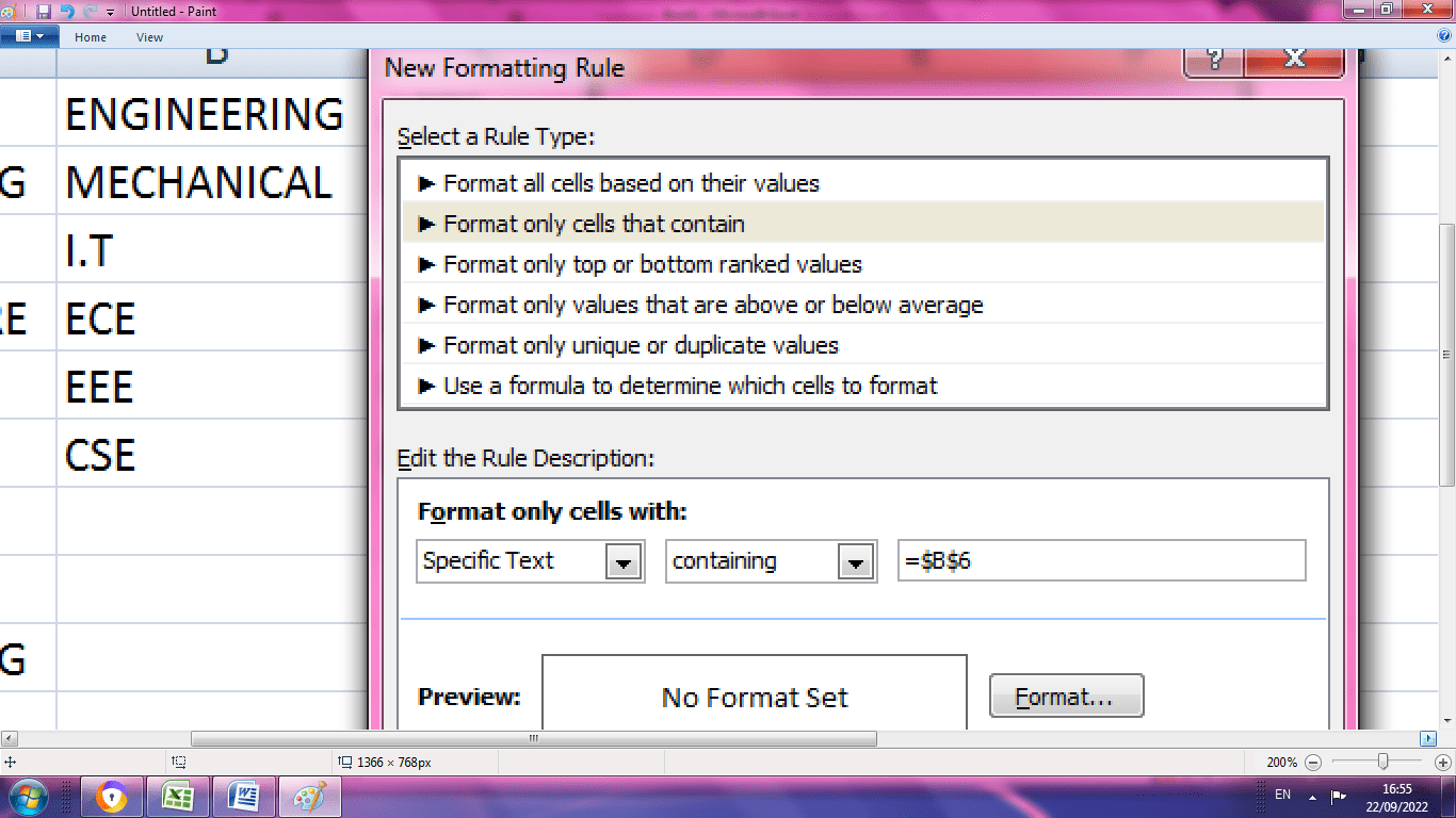
STEP 5: In the new formatting Rule dialogue box, select "Format cell that contains", and under the division, choose “Specific text” in the first drop-down list "containing" displays in a default manner and select the required cell in the third dialogue box.

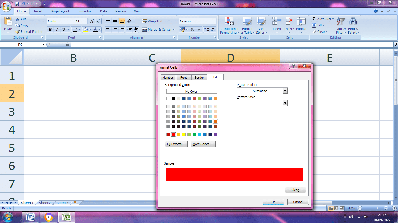
STEP 6: In the fill option, choose the required colour and click ok.

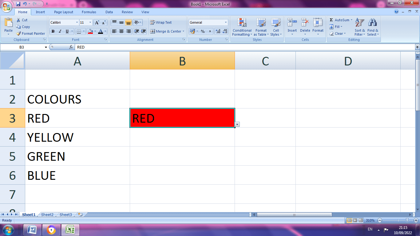
STEP 7: Finally, the cell appears as the user's choice of color

.

Features of Drop-down list

• The spreadsheet looks more efficient by providing the spreadsheet
• Data entry is quicker and more accurate when we opt for a drop-down list.
• It limits the data entries in the cell.
• When the cell is selected, the drop-down list appears, and the user can choose the Data easily.