Averageif Function in Excel

Average If in HTML

In Mathematics, Average function is used to find the arithmetic mean of the given data. It is defined as the dividing the sum total of given data by the number of data.  Microsoft excel provides default functions and formulas for calculation purposes. The function name called AVERAGE which handles of about 255 individual arguments like ranges, arrays, numbers, cell references and constants. It helps to retrieve the average of the given data.

Average Function in Excel

Excel provides a default function called Average to find the average of the given data.

Formula Used

The syntax for the average function is as follows,

=AVERAGE (number 1,[number2],…)

Number 1 – It represents the number or cell references which refer to numeric values.

Number 2- This parameter is similar to number 1 which is an optional one.

To find the average of the given numbers, it sums all the numeric data and divides by the count of numeric values. The function AVERAGE can take the arguments such as number 1, number 2, number 3 etc. It avoids the empty cells and cells which contains text or logical values. If the input is error, AVERAGE function returns error.

Example 1: How to calculate the average for the given data in Excel?

Step 1: Enter the data in the worksheet which is represented in the form of rows and columns.

Step 2: Select a new cell where the result wants to display and enter the formula as =AVERAGE (CELL RANGE). Here cell range indicates the data present in the cell.

Step 3: The average will display in the respective cell. To find the average for all the data, drag the formula towards the entire cell which contains data. It displays the result for the entire data.

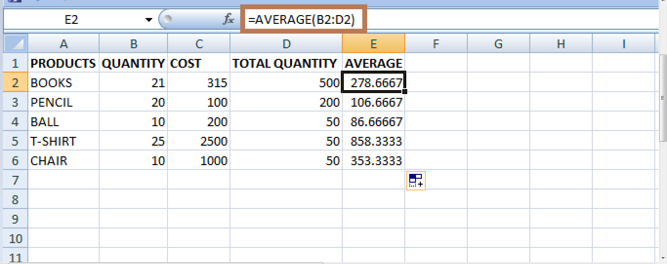
From the above spreadsheet, the average for the given value is calculated using AVERAGE function.

Example 2: How to calculate the average function for blank cells?

While performing average calculations in Excel, what will the function do if blank cell is present in the table? The average function ignores the empty cell and performs the calculations for the remaining values.

Step 1: Enter the required data in the table, where there contains as empty cell.

Step 2: Select a new cell, where the result wants to display and enter the formula as = AVERAGE (cell range).

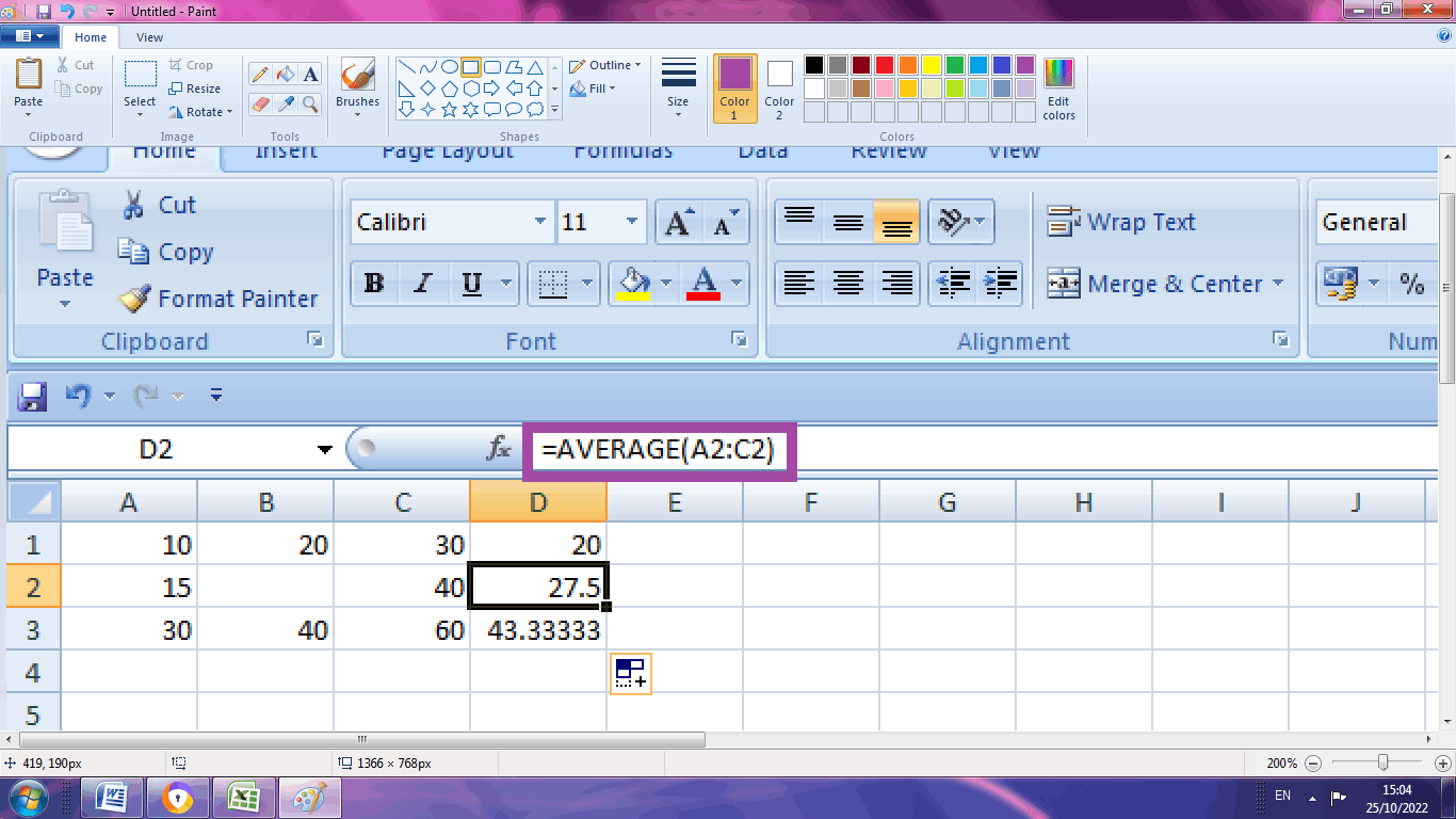
Here in the above example, the average value for the cell A1:C1 is calculated first, where the result will display in the cell D1. Drag the formula towards the cell D3, where the result will displayed for remaining data. Here the cell B2 is empty, the formula ignores the empty cell and calculates the average for B1 and B3.

Example 3: How to exclude empty cell while calculating the average function?

Sometimes the data tables contain zero or empty values. To exclude the empty cell or zero values, Excel provides default function called AVERAGEIF or AVERAGEIFS is used. To use this function,

Step 1: Step 1: Enter the required data in the table, where there contains as empty or zero value cell

Step 2: Select a new cell, where the result wants to display and enter the formula as = AVERAGEIF (cell range,”>0”) where the formula represents to exclude zero.

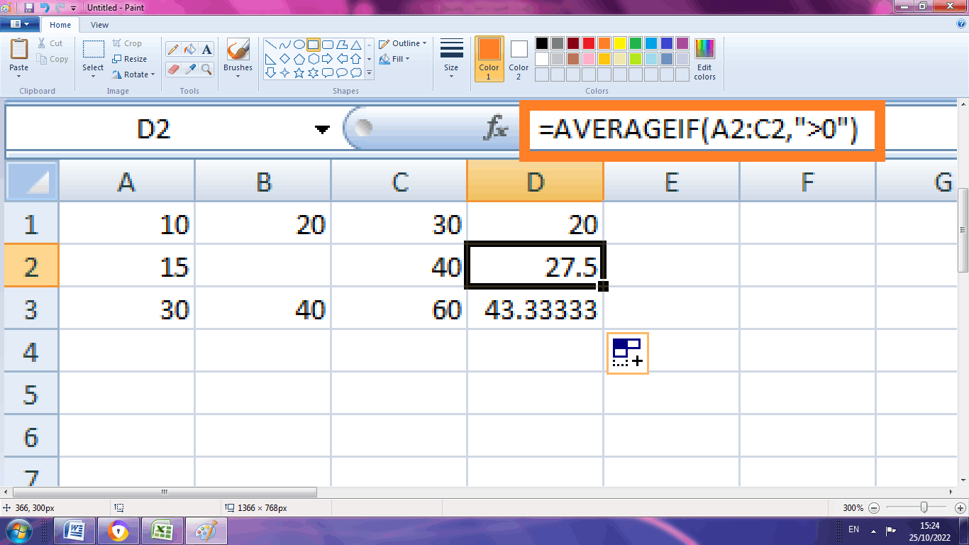
Here the formula excludes the zero value while calculating the average for the values. Similar to AVERAGE, AVERAGEIF excludes the empty cell or zero values in default manner.

Example 4: How to calculate the average function for Mixed Values?

Usually the average function is calculated based on values which are present in row wise and column wise. Sometimes it needs to be calculated in mixed values.

Step 1: Enter the required data in the worksheet.
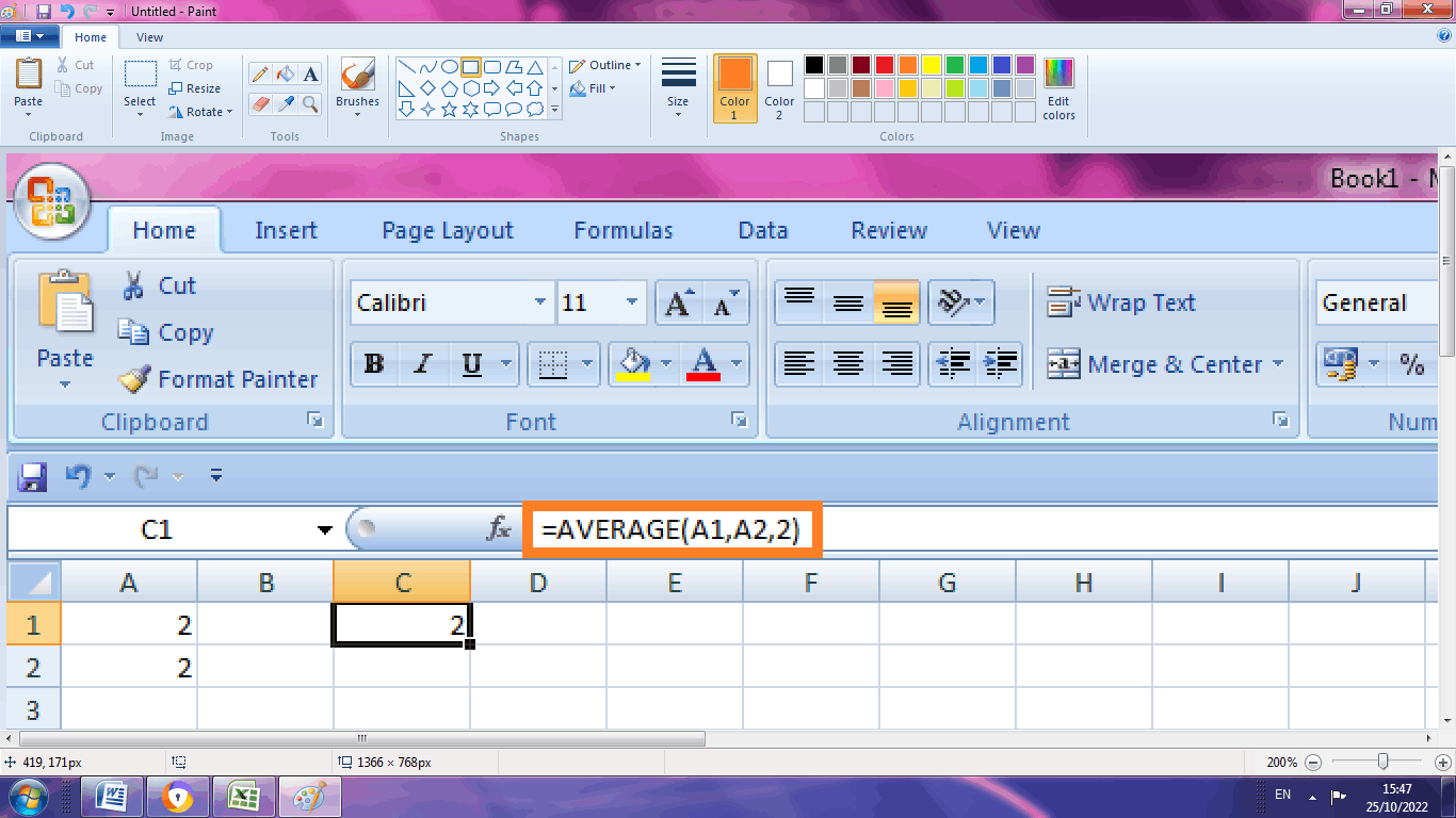
Step 2: Here in this example, the average is calculated for the cell A1, A2. Select a cell and type the formula as =AVERAGE (A1, A2, 2). The number ‘2’ represents the user’s choice of value which is added as the third argument to calculate the average.

Example 5: How to calculate average based on certain criteria or conditions?

The data contains mixed group of value, sometimes there is a need to calculate the average function based on certain conditions. Here is an example,

Step 1: Enter the data which contains the students mark and their class as follows,

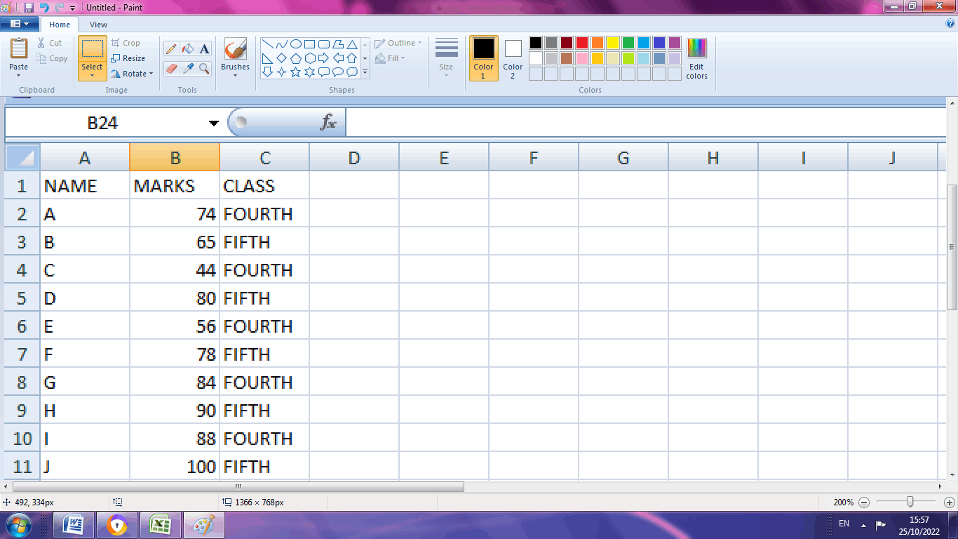
From the above given data, the average needs to be calculated individually for the students who are studying in fourth grade and fifth grade

Step 2: To calculate this AVERAGEIFS function is used. Select a cell and type the formula as =AVERAGEIFS (B2:B11, C2:C11,”FOURTH”).

Step 3: Similarly select another cell and type the formulas as =AVERAGEIFS (B2:B11, C2:C11,”FIFTH”).

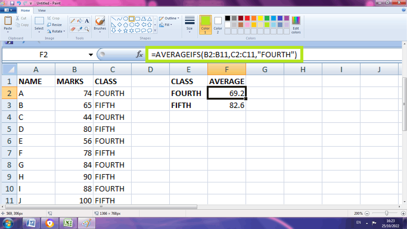
The results are displayed in the respective cell individually for fourth and fifth grade.

Example 6: How to calculate the average of top ‘n’ values for average function?

Here in this example, the steps are explained how to calculate the average for top ‘n’ values.  To calculate the top ‘n’ values LARGE function is used.

Step 1: Enter the set of data in row and column wise.

Step 2: Calculate the normal average function for the data using the formula =AVERAGE (CELL RANGE). Similarly calculate the average function for the remaining data by dragging the formula down.

Step 3: For example to calculate the average for top three values, select the cell and enter the formula as =AVERAGE (LARGE (CELL RANGE, {1, 2, 3})). The formula calculates the average for the top three values present in the row.

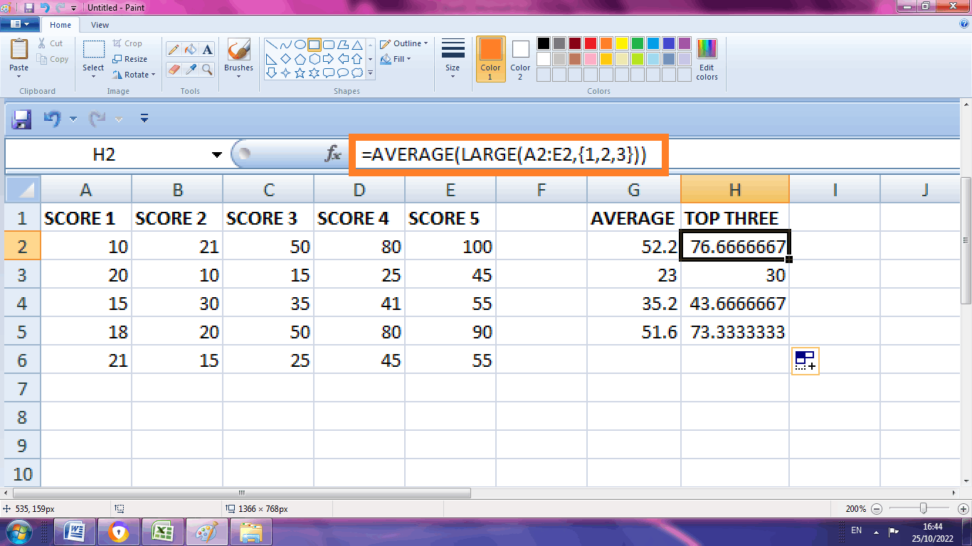
From the above worksheet, the average for top three values in every row is calculated. For example the average for row A2:E2 is calculated by adding the values of (100, 80, and 50) and divided by 3 where the result is obtained as 76.6. Similarly every top three value is calculated.

Weighted Average

To calculate the weighted average for the data, Excel provides the default function called SUMPRODUCT function is used. Here is an example to calculate the weighted average function for the following data.

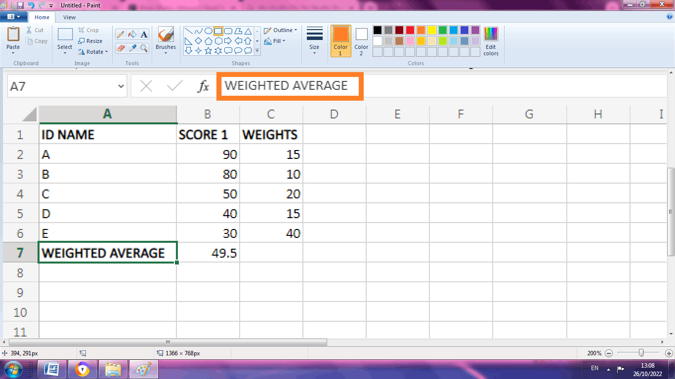
Step 1: Enter the required data in the worksheet in the respective rows and columns. Here score and their respective weights are entered in the respective column

Step 2: To calculate the weighted average, select a cell and type the formula as =SUMPRODUCT (weights, cell range)/SUM (weights). The formula entered by selecting the cell range =SUMPRODUCT (B2:B6, C2:C6)/SUM (C2:C6). The weighted average will display in the respective cell as shown below.

Example 7: How to calculate the average using certain criteria?

Here based on certain criteria, the average is calculated using the function called AVERAGEIF.

Here is an example how to calculate the average based on the selective data

Step 1: Enter the data in the spreadsheet.

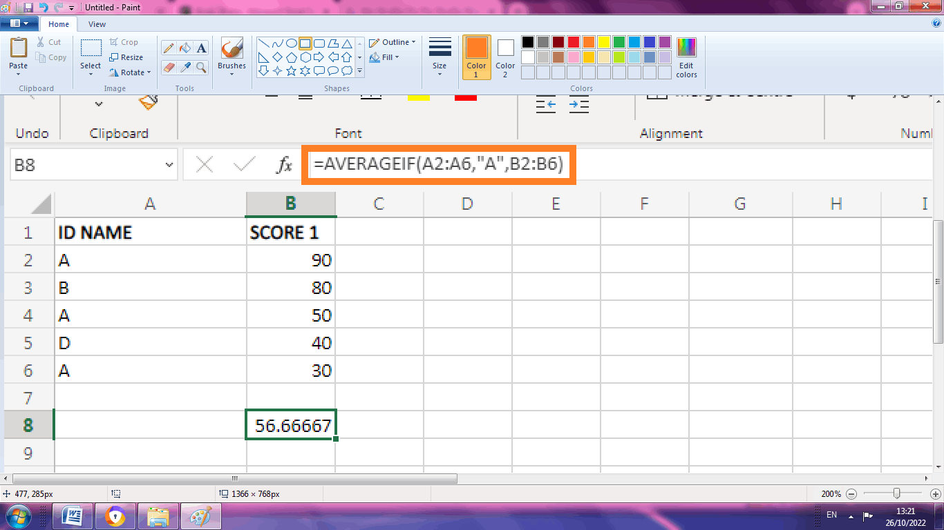
Step 2: Select the cell where the result want to display and enter the formula as =AVERAGEIF (A2:A6,”A”, B2:B6). Here this function calculates the average for the value “A” only which is selected. The result is based on the values (90, 50, and 30). To apply some conditions or criteria AVERAGEIF is used.

Example 8: How to exclude some values using Average Function?

Step 1: Enter the respective data in the rows and columns.

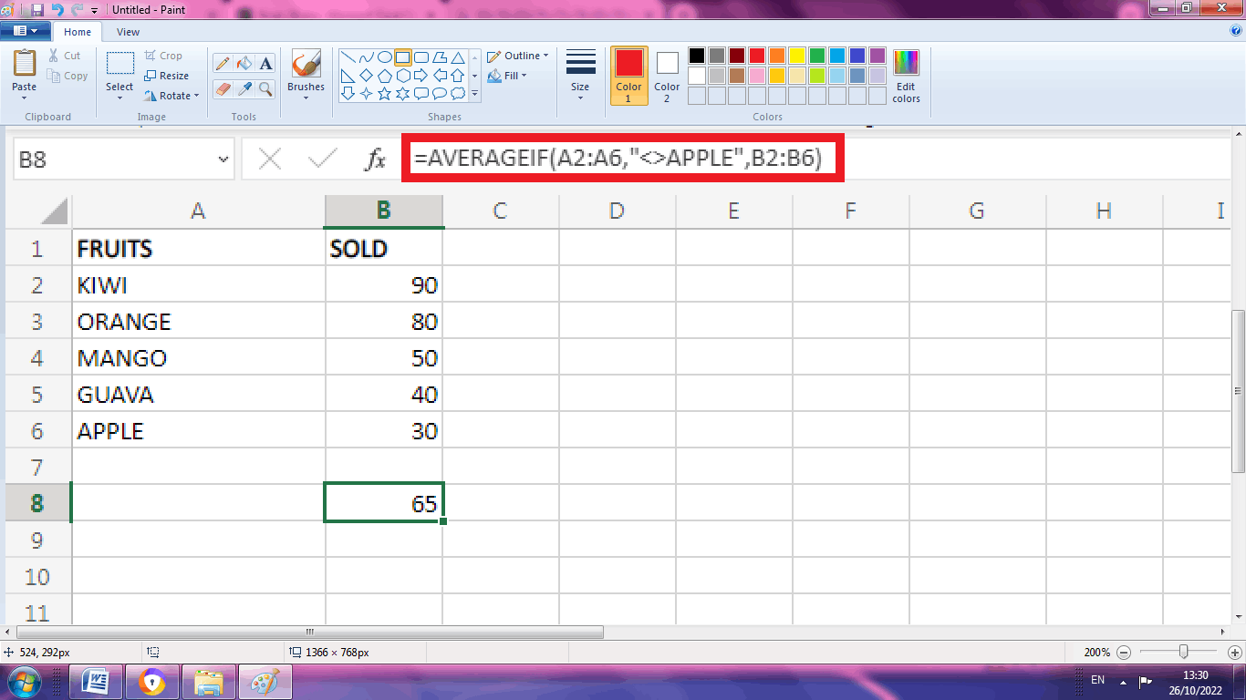
Step 2: From the above chart enter the formula as =AVERAGEIF (A2:A6,”<>APPLE”, B2:B6). Here the data value called “APPLE” is excluded while calculating the average function. The result is displayed based on the result (90, 80, 50, and 40) where the value of APPLE is not added.

Example 9: How to calculate the average function based on certain selective characters?

To calculate the average based on certain selective characters, the steps to be followed are,

Step 1: Enter the data in the spreadsheet.

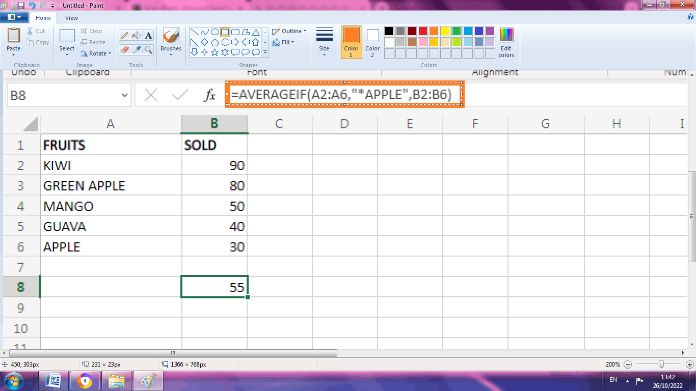
From the above worksheet, the formula =AVERAGEIF (A2:A6,”*APPLE”, B2:B6) calculates the value which contains the series of zero or various characters+ APPLE. Here in this formula (*) matches a series of zero or various characters.

 Example 10: How to calculate the average function for selective data or characters?

Sometimes the average needs to be calculated for certain selective data or characters. For example, here is an example how to calculate the average for ‘5’ letter character.

Step 1: Enter the data in the spreadsheet.

Step 2:  Select a cell, where the result wants to display, and enter the formula as =AVERAGEIF (A2:A6.”?????”, B2:B6). Here the “?????” indicates the four letter character present in the data.

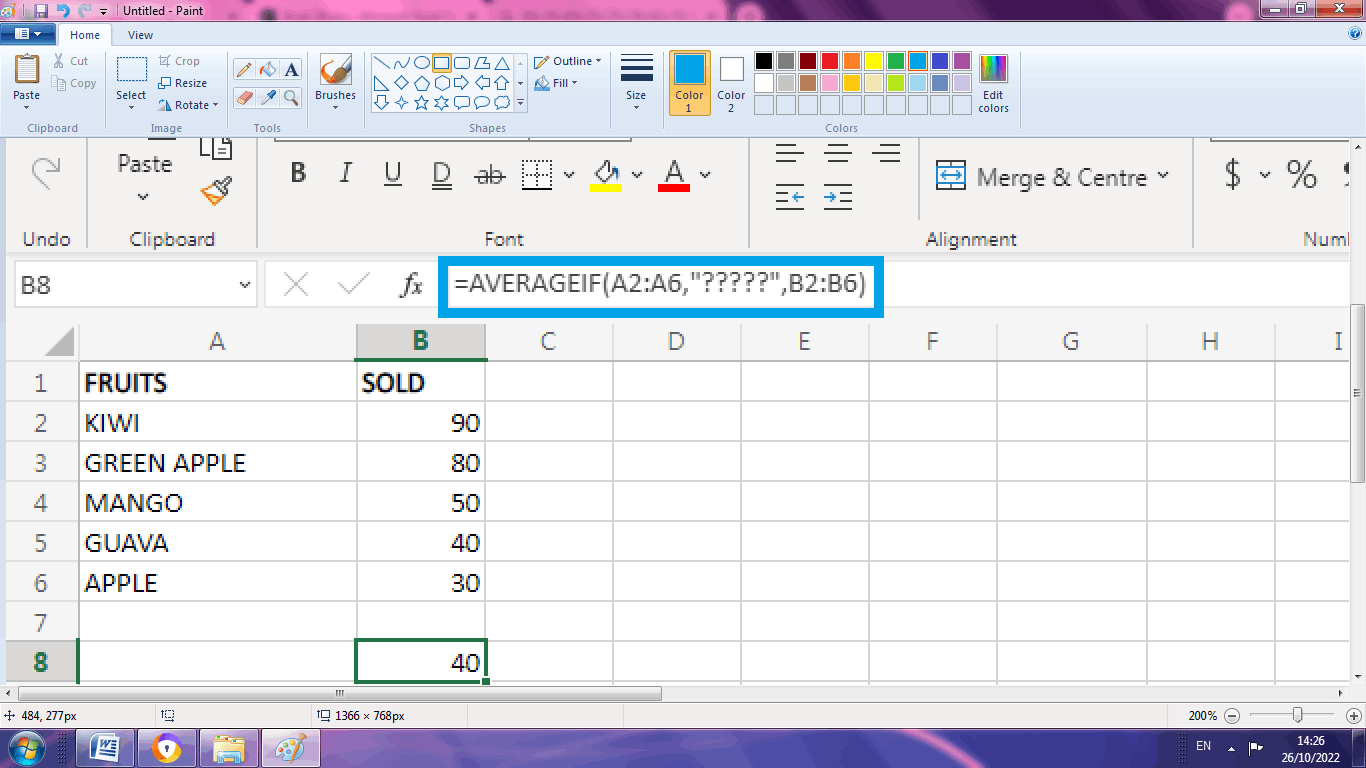
From the above worksheet, the average is calculated for data which contains the character “5”. A single question mark (?) matches only one character. Based on the user’s choice of character the question mark is placed.

Example 11: How to calculate the average with the selective value conditions?

Here is an example, where the average is calculated based on certain conditions.

Step 1: Enter the data in the spreadsheet.

Step 2: Select the cell where the result want to display and enter the formula as =AVERAGEIFS (A1:A5, A1:A5,”>=100”, A1:A5,”<=500”). Here condition is applied to calculate the average for the values which is greater than 100 and lesser than 500.

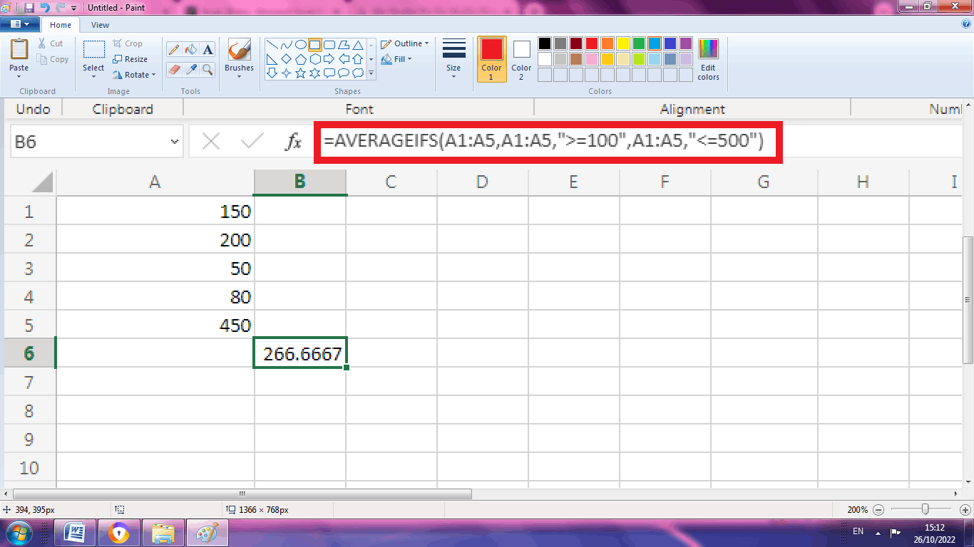
Here in the above worksheet AVERAGEIFS function is used where the letter ‘S’ at the end calculates the average of the cells which meets multiple criteria.

Example 12: How to calculate the average for the selective data pairs?

To calculate the average for the selective data pairs, following steps are followed.

Step 1: Enter the data in the spreadsheet

Step 2: Select a new cell, and enter the formula as =AVERAGEIFS (C1:C5, A1:A5,”Mango”, B1:B5,”PINEAPPLE”) .Here the average is calculated for Mango and Pineapple data.

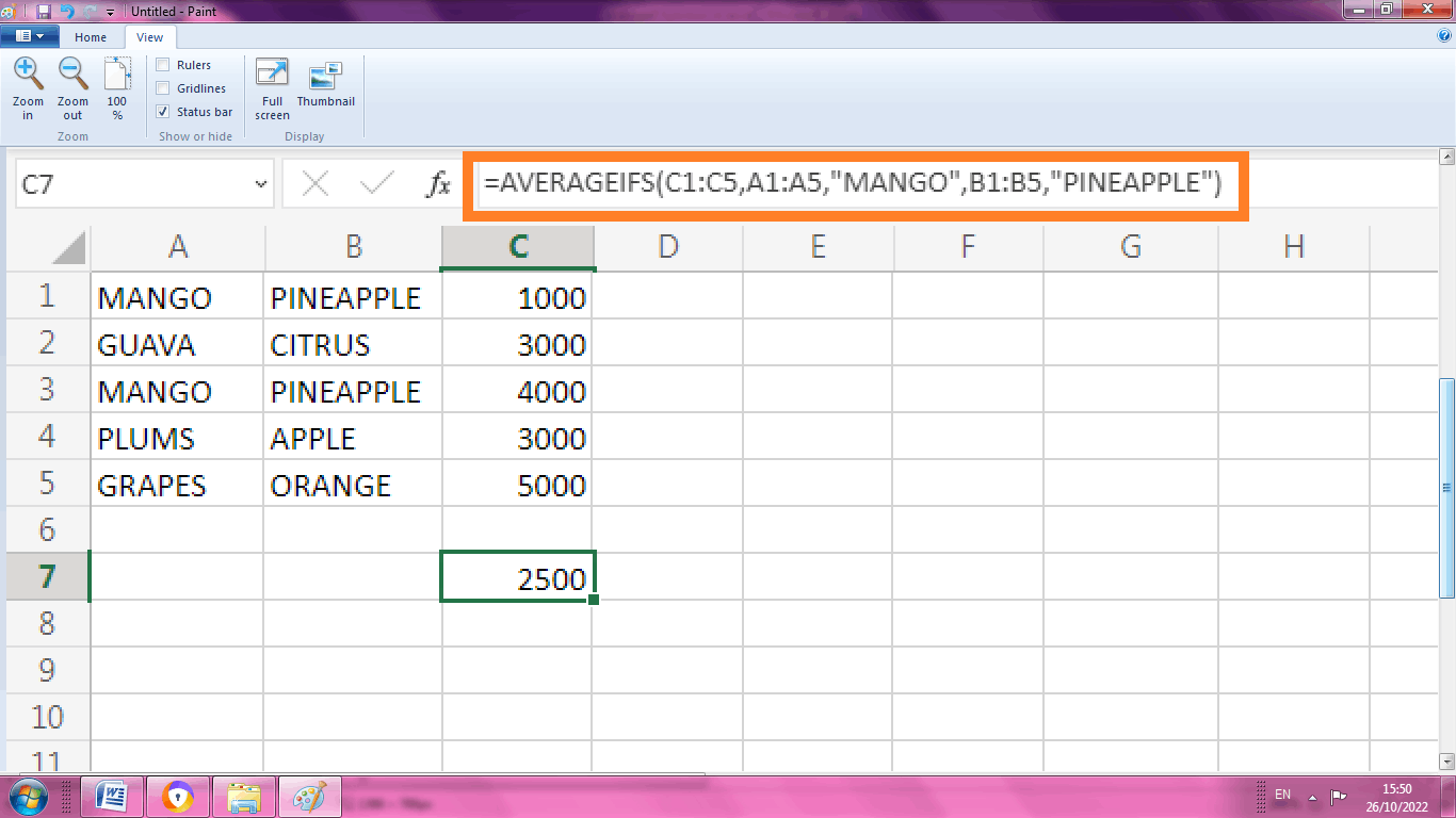
From the above worksheet the multiple criteria is applied, by choosing the cell that contains Mango and Pineapple using default AVERAGEIFS function

Summary

From the above tutorial, the various functions and formulas for Average IF function is explained briefly.