Microsoft Excel is used for multiple purposes in various organizations. It is a combination of numeric values, alphabets etc. To calculate data, the user organizes the data according to their convenience using the Excel default function. Excel consists of various in-built functions that help organize and review the data quickly and efficiently. While calculating and finalizing the data, the user needs to check the duplicate or repeated value, the difference between the data called row difference. Calculating the row difference is one of the tasks which is done by the Excel default feature. Here in this tutorial, the steps to calculate the row difference are described in a step-by-step method.

1. How to find the row difference in Excel?

If the row difference is highlighted, the user’s time is saved during calculations. To highlight the row difference first find the difference between the data, to highlight the data, formatting method is applied. Highlighting the data helps to update, review, or analyze the data in future easily and quickly.

The steps to be followed for finding the row difference is as follows,

Step 1: Enter the data in the spreadsheet in the respective row and column.

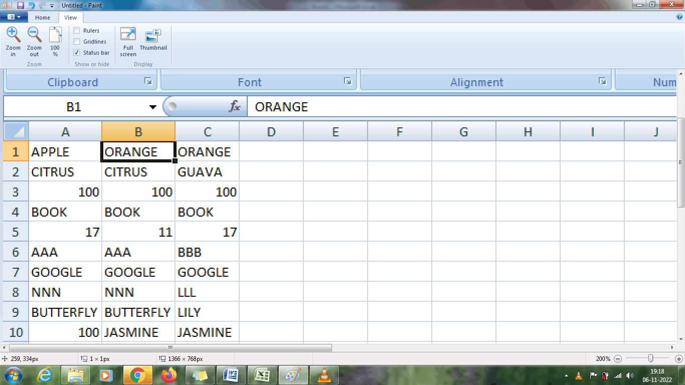
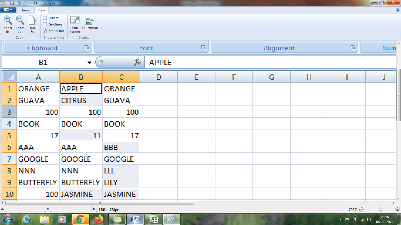
Step 2: To select the cell range from A1:C10, select any cell, here the cell A1 is selected. After selecting the cell drag the arrow mark towards the cell C10. Here the cell A1 is called active cell. Selected active cells present in the column (here A1 is selected), which needs to be compared with the correspondent row. For example the value present in A1 is compared with the value B1 and C1. Likewise the values present in the column range A1:A10 acts as a comparison values.

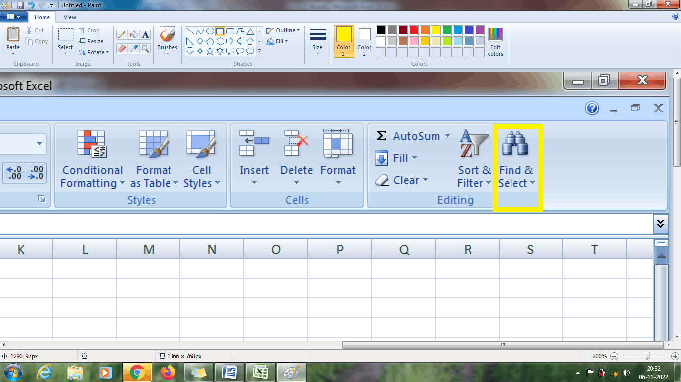
Step 3: Select Find and Select option in the Editing Group from the Home Tab.

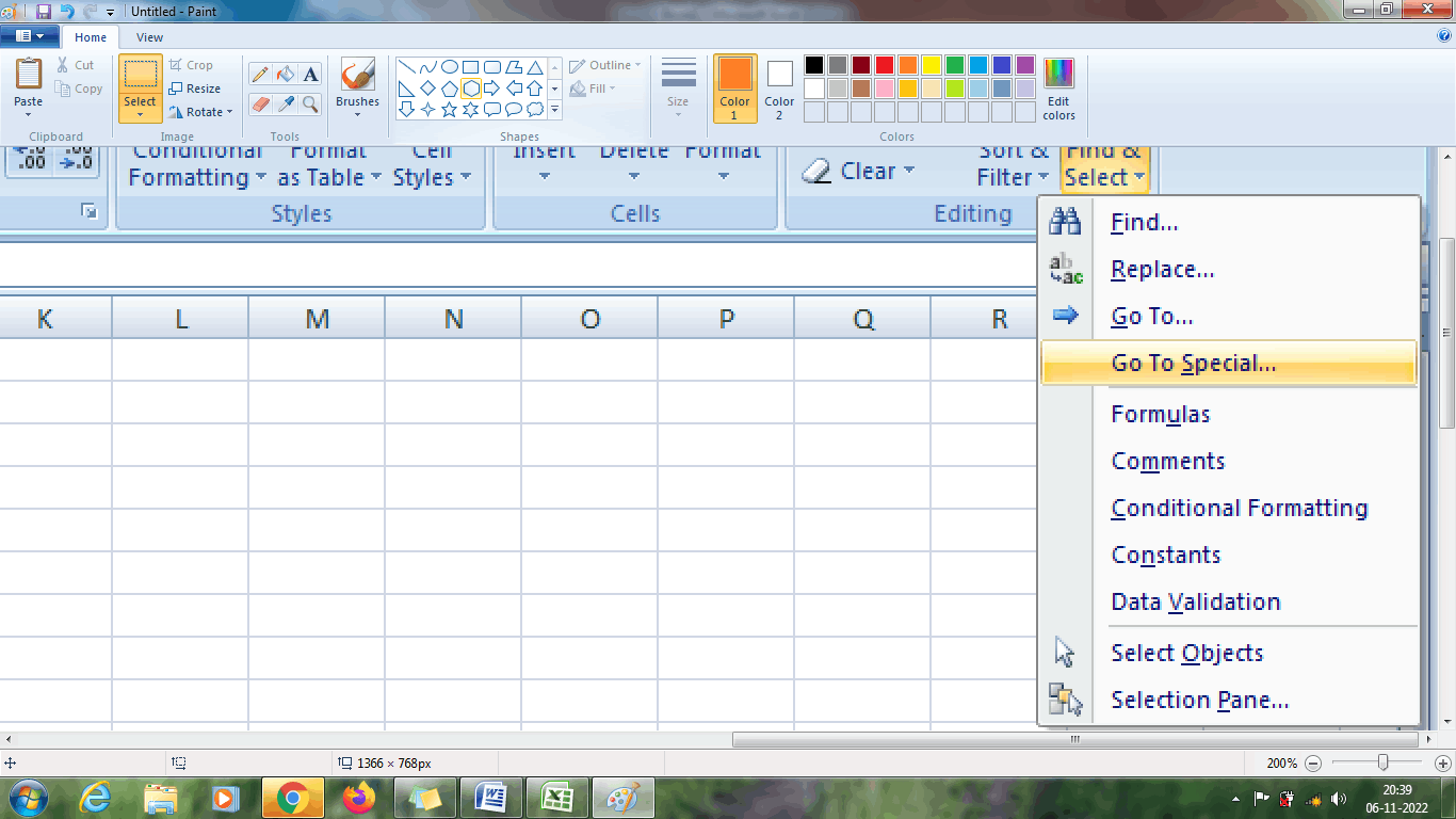
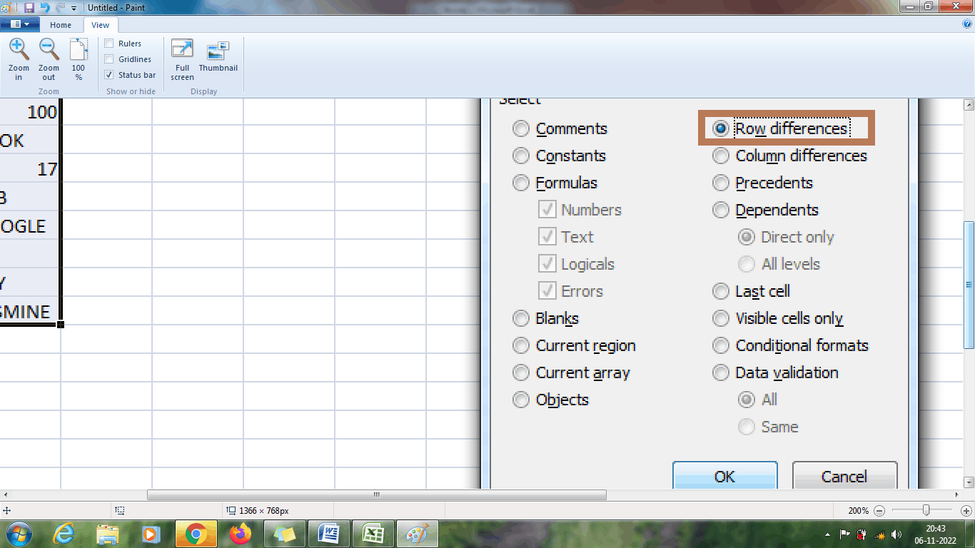
Step 4: Choose the “Go to Special “option.

Step 5: Choose the Row Difference and click Ok.

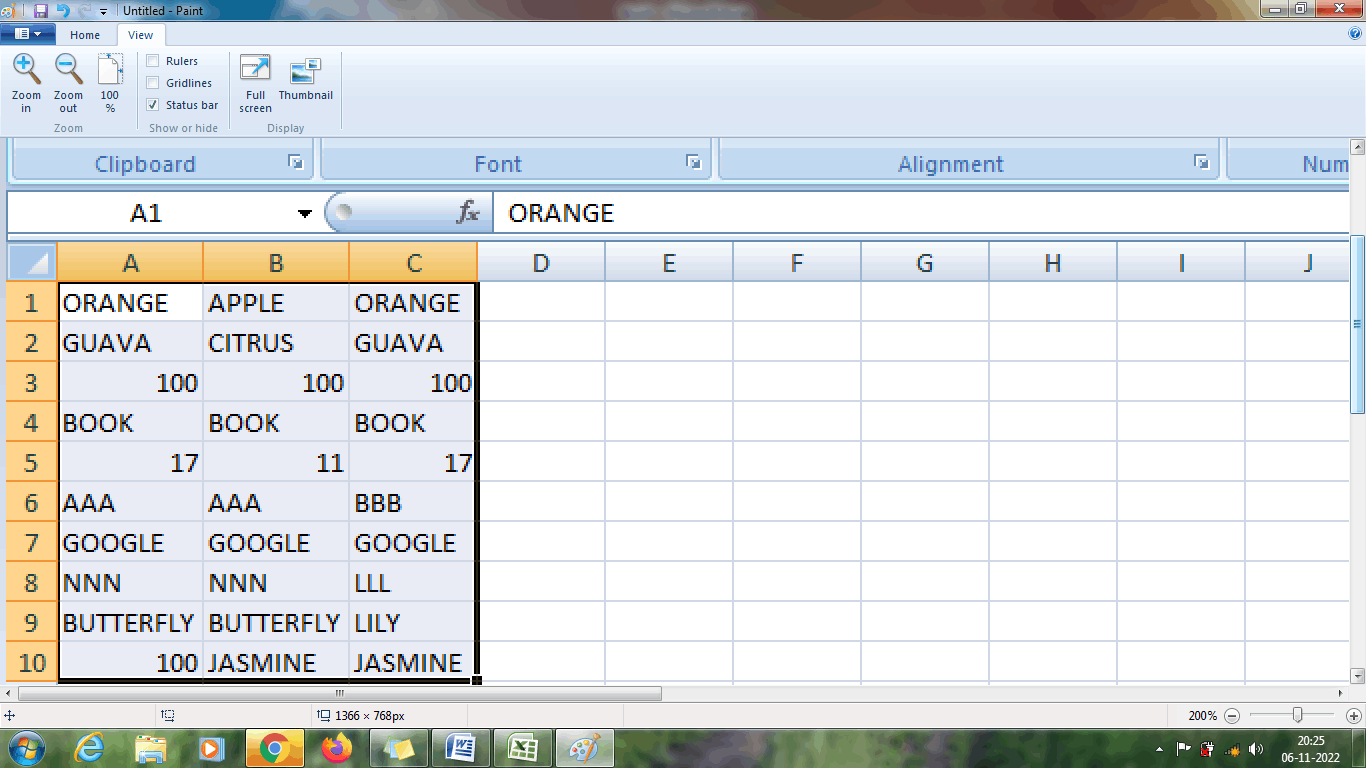
Step 6: The cell difference is highlighted comparing with the values present in the column A1:A10. From the above cell, the value in B1 varies compared to A1. B2 vary compared with A1. B5 vary compared with A5. C6 vary with A6. C8 vary with A8. C9 vary with A9. B10 and C10 vary with A1. Therefore the cell difference is highlighted.

2. How to change the background colour of the highlighted cell?

To set the desired background colour to the highlighted cells, the steps to be followed are,

Step 1: After finding the cell difference, change the background colour from the font group in the Home Tab as shown in the image.

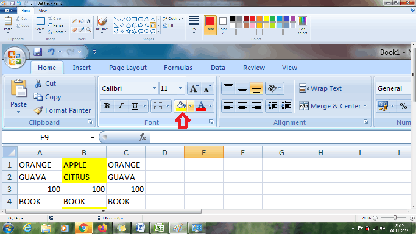
Step 2: Fill the necessary colour in the font group. The selected colour is applied to the highlighted cells. This helps to view the highlighted cells easily and quickly while organizing and calculating the data.

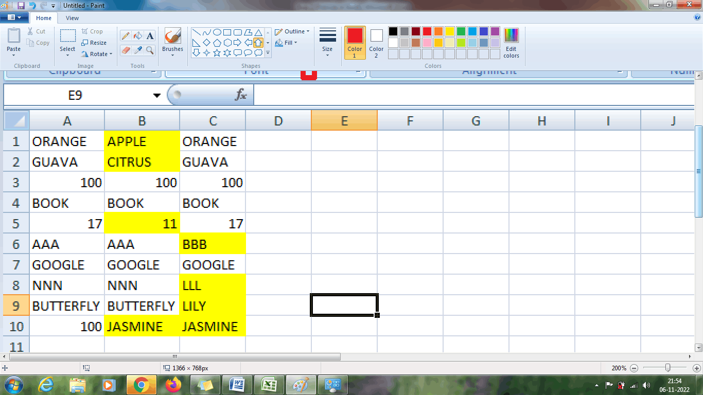
From the above worksheet, the row difference is highlighted in yellow in color.

3. How to compare two columns using formula?

To compare two columns, in Excel using row by row the IF formula is used. The formula is used to compare two cells in the respective row. The steps to be followed are,

Step 1: Enter the data in the respective row and columns namely A1:B7.

Step 2: Choose a new cell where the result wants to display namely C1 and enter the formula as =IF (A1=B1, “Match”,””). The result will be displayed in the cell C1.

Step 3: To display the result in the respective cells, drag the formula towards the cell C7. The result will be displayed in the remaining cells whether the data present in the cell is matched or not.

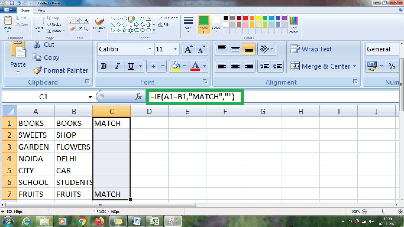
From the above worksheet, if the value matches, the result is displayed as MATCH.

If the user wants to display the result as “No Match”, then type the formula as =IF (A1=B1, “MATCH”,”NO MATCH”)

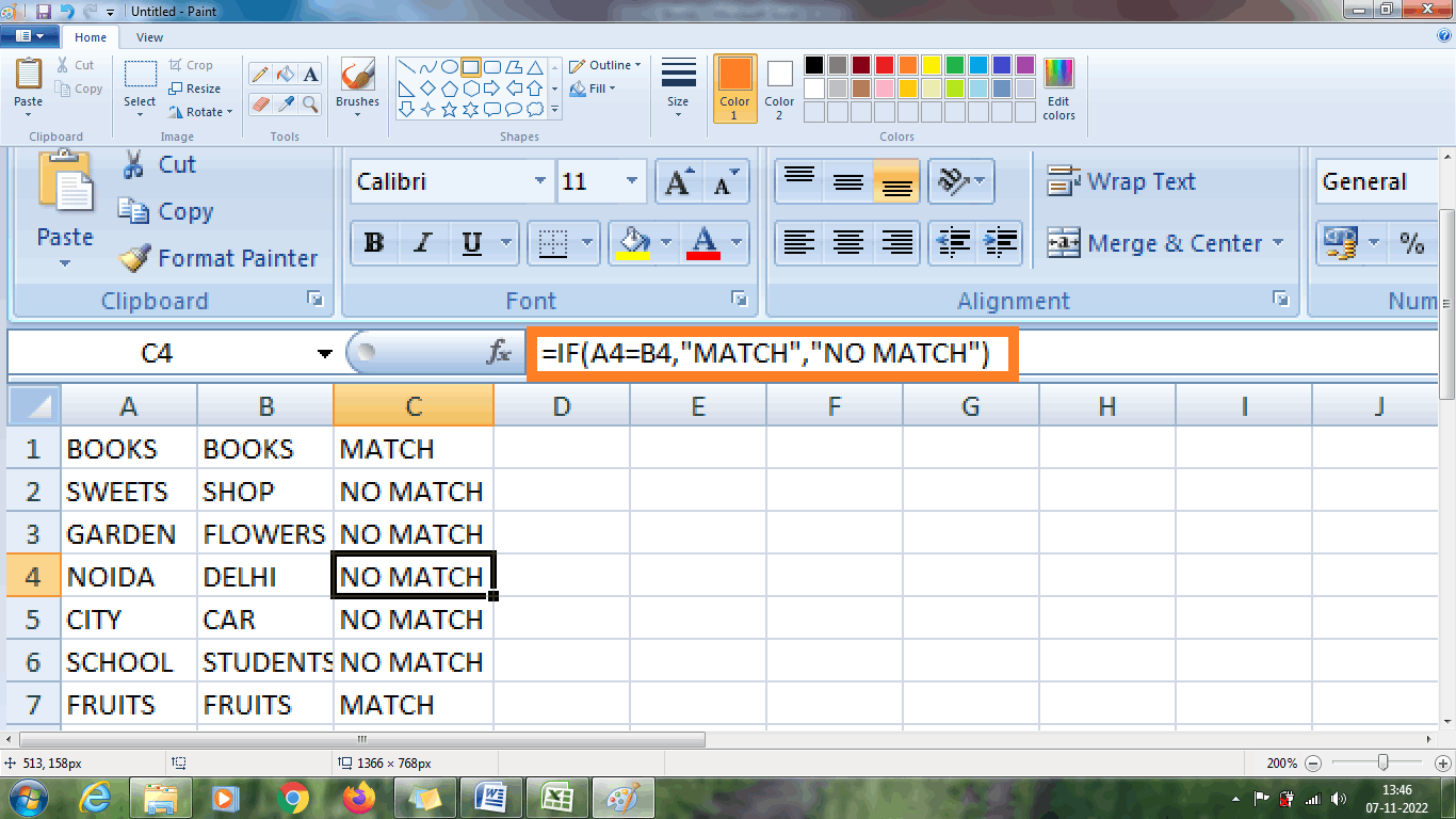
From the above images, “NO MATCH” is displayed as result, if the value does not match.

4. How to compare the case-sensitive data?

Sometimes the user needs to compare the two columns, whether the respective column contains data which is case sensitive or not. To find the case sensitive data, the EXACT function is used. The steps to be followed are,

Step 1: Enter the data in the respective row and columns namely A1:B7.

Step 2: Choose a new cell where the result wants to display namely C1 and enter the formula as =IF (EXACT (A1, B1),”Match”,””). The result will be displayed in the cell C1.

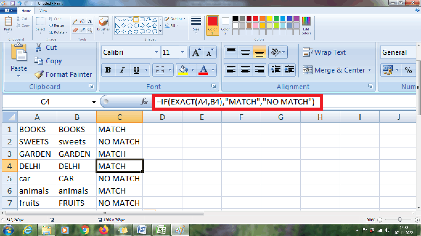
From the above worksheet, the result is displayed as “MATCH” if the data matches, and “NO MATCH” is displayed if there occurs a case-sensitive difference in the data. To find the case-sensitive differences, the formula is modified as =IF (EXACT (A1, B1),”MATCH”,”UNIQUE”). The result UNIQUE will be displayed, if there occurs a data difference in case-sensitive.

5. How to compare multiple columns in Excel?

If the table contains multiple columns, to find the rows which consists of similar data in all the cells, the IF formula with AND statement is used. The steps to be followed are,

Step 1: Enter the data in the respective row and columns namely A1:C7.

Step 2: Choose a new cell where the result wants to display namely D1 and enter the formula as =IF (AND (A1=B1, A1=C1),”Full Match”,””). The result will be displayed in the cell D1.

Step 3: To display the result in the respective cells, drag the formula towards the cell D7. The result will be displayed in the remaining cells whether the data present in the cell is full matched or not.

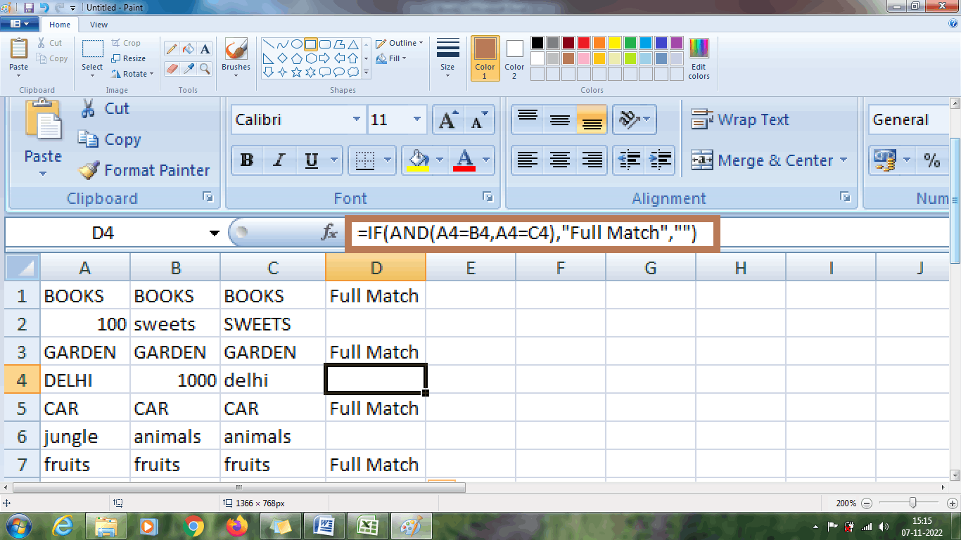
From the above worksheet, the result “FULL MATCH” indicates that the data is fully matched and empty cell indicates that the cell is not fully matched.

6.How to find the matches in any two cells in the same row?

Sometimes the data contains multiple rows and columns. To find the row match between any particular cells among various cells, the steps to be followed are,

Here in this example among 7 rows and 4 columns, the data matches between three columns is found in this example.

Step 1: Enter the data in the respective row and columns namely A1:D7.

Step 2: Choose a new cell where the result wants to display namely E1 and enter the formula as =IF (OR (A1=B1, B1=C1, A1=C1),”Match”,””). The result will be displayed in the cell D1. Here the column A, B and C are compared.

Step 3: To display the result in the respective cells, drag the formula towards the cell E7. The result will be displayed in the remaining cells whether the data present in the cell is matched or not.

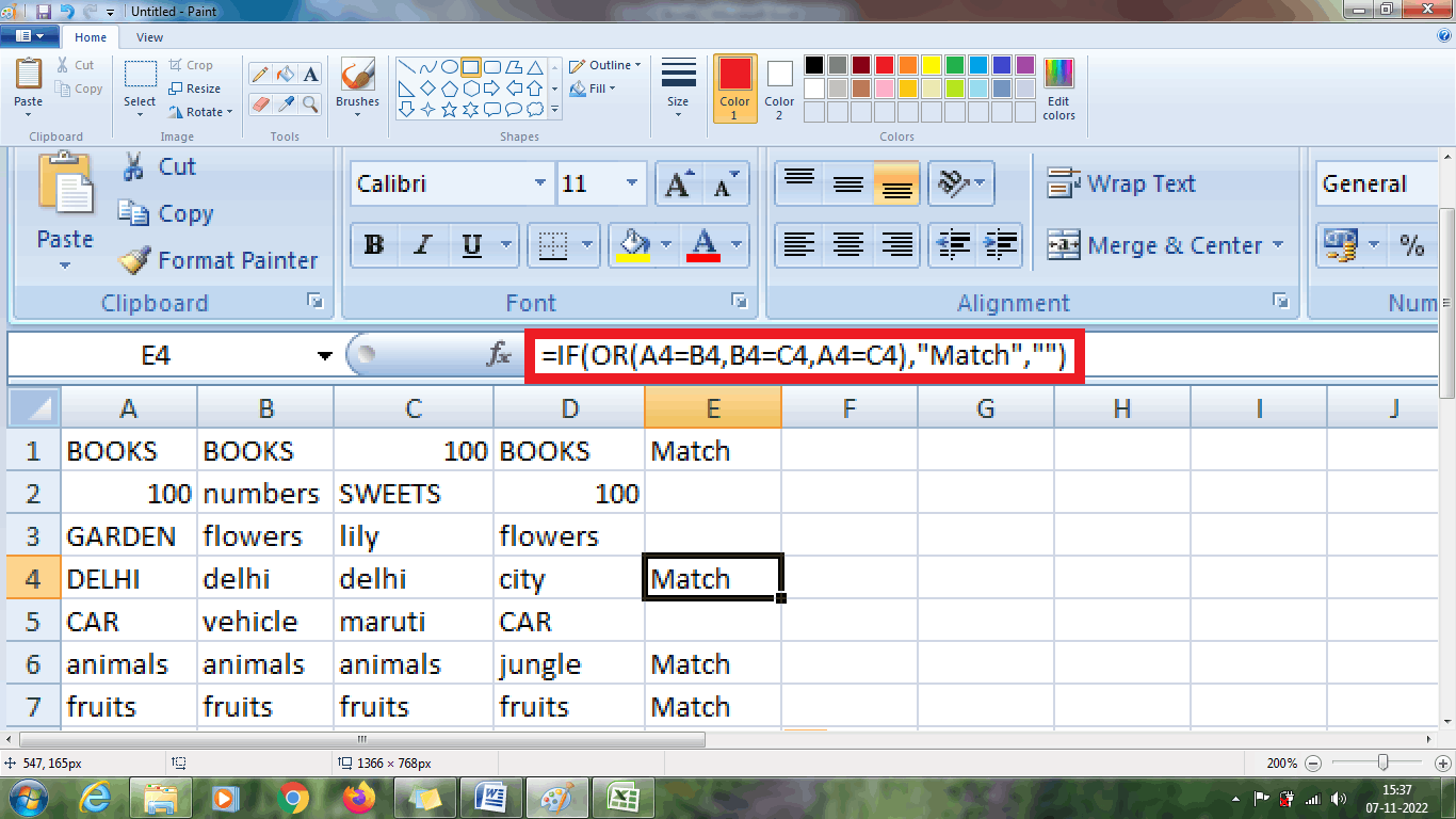
From the above worksheet, the result is displayed as “Match” any one of the condition is true such as A1=B1, B1=C1, and A1=C1. Hence to check multiple columns, the required condition is applied in the IF and OR to check the data similarities.

Summary

From the above tutorial, the various functions and methods of finding the Excel row differences and matches is explained briefly.

Excel Tutorial

Functions

How To

Misc