SumIF Formula in Microsoft Excel

SUMIF Formula in Microsoft Excel is considered the primary and vital formula individuals can use to remove their workload.

In this tutorial, we will discuss and learn about the SUMIF Formula used in Microsoft Excel; besides all these, we will also look into the use of the function with various examples.

What do you mean by the term SUMIF Function?

“The Sum function primarily adds the number values or all the numerical cells data specified in a range. An individual uses the SUMIF process to add cells or a range when some specific type or the appropriate criterion gets met.”

Thus, we can say that this function adds all the present cells of the excel sheet that fulfil the certain defined conditions and criteria, respectively. Moreover, the measures could be any of the following such as:

1. Text.
2. Number.
3. And the Logical operator.
4. Etc.

In short, we can define it as the conditional sum of the cells in a particular sheet of Microsoft Excel.

Furthermore, this specific function is the worksheet function, ideally available in all the updated versions of Microsoft Excel. And they can be categorized under the Math and Trigonometry formulas.

How to make use of SUMIF Formula in the Excel sheet?

=SUMIF( 
     SUMIF(range, criteria,[sum_range])

The formula as mentioned above is termed to be the syntax, and it has various arguments which are, as discussed in brief below, effectively,

1. Range: The range in Excel is considered to be the required argument. It is the cell range on which the particular condition or the criteria is applied. The cell of the respective Excel sheet must contain the various numbers, dates, and text, as well as the cell references with numbers. And in this case, if the cell is blank, it does not contain any data on it and must be ignored effectively.
2. Criteria: The criteria are considered to be the required arguments and are defined as the criteria that will effectively decide which cells need to be added.

In other words, it is termed to be the condition based on which the cells will be summed up respectively, and the criteria can be of various things such as:

1. Number.
2. Text.
3. Multiple dates in excel formats.
4. Logical Operators.
5. And the cell references.
6. Etc.

For example: 7, “Harish”, C13,”<6”,, 09/09/2022, etc.

• Sum_Range: Sum_Range is termed to be the cell range that needs to be get added. And these are also considered to be the arguments in the excel sheets that are optional, and they are the individual cells that differ significantly from those in the range.

Besides these, if an individual arises with the case where there is no sum range, then in that case he might add the original cell range respectively.

Use of SUMIF Formula in the Microsoft Excel

The SUMIF formula is primarily straightforward to use by anyone who wants to simplify the data. Let's get started with the help of a practical and simple example related to the SUMIF.

In the below example, we have considered only one column or range respectively,

# Example 1:

This example is very much bare as they consist of only two arguments.

Below is the attached screenshot; there is the single column data on which we will make use of the function that is "SUMIF Function." We efficiently need to add the individual cells above or could be > 20 in the cell range from A1 to A8 (A1:A8).

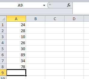
After that, we will now, in the further steps will, write down the respective type of the formula in the particular cells that are none other than the A9 cells. This will differ from the various data that an individual uses.

As depicted in the below-attached screenshot.

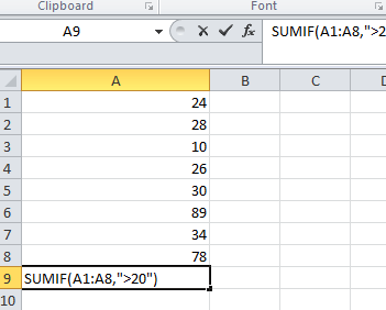
In this, we have seen that the range "A1:A8", criteria are ">20", and then since, it was made under noticed that there is no sum_range so the cell of the respective range (A1:A8) will get added, which are seen in the below-attached screenshot.

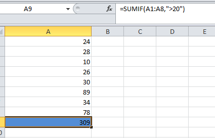
In the above screenshot, the numbers above 20 are added and below 20 are primarily excluded.

Furthermore, we can use the cell reference as the condition and the criteria instead of hard-coding for the actual value.

As depicted clearly in the below-attached screenshot.

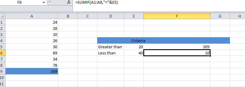
This is how we can effectively use the cell references as the condition or the criteria instead of writing them separately.

# Example 2:

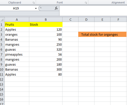
In this respective example, we have collected the data set of various types of fruits as well as their stock, shown below in the attached screenshot. Let us assume that we want to calculate availability of the stock for the fruits, that is, "oranges."

And for this, we will write down the formula in the respective cell, cell E3. As depicted in the below-attached screenshot.

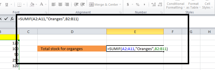
The arguments which are used in the above formula are explained below in detail,

•   Range: The range in Excel is considered to be the required argument. It is the cell range on which the particular condition or the criteria is applied. The cell of the respective Excel sheet must contain the various numbers, dates, and text, as well as the cell references with numbers.
• And in this case, if the cell is blank, it does not contain any data on it and must be ignored effectively. As per the above example: A2:A11, in this particular range, the condition or the criteria of mangoes shall be applied successfully.

• Criteria: The criteria are considered to be the required arguments and are defined as the criteria that will effectively decide which cells need to be added.

In this example, it is oranges for which we want to calculate or know the sum of all the oranges out of the fruits present.

• Sum_Range: Sum_Range is termed to be the cell range which needs to be added. And these are also considered to be the arguments in the excel sheets that are optional, and they are the individual cells that differ significantly from those in the range.

Besides these, if an individual arises with the case where there is no sum range, then in that case he might add the original cell range respectively.

As per the above example: The sum_range in this respective example would be B2:B11.

And to get the desired output or the result, we should press enter, and the result will appear on the screen. As shown in the below-attached screenshot.

Output:

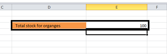
And we have the output, which we have, totalling 100 oranges.

# Example 3:

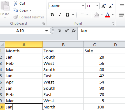
Let us consider the other example in which we have data related to sales from the various zones. And we want to know or calculate the total sales from the South Zone, as depicted in the screenshot below.

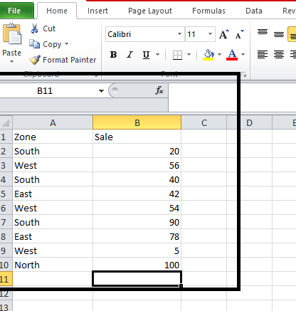
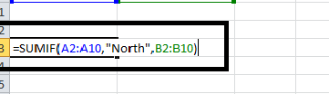
Now, we will move on to writing the formula in the cell that is B12, as documented below effectively.

• Range:  The range could be from A2 to A10.
• Criteria: North
• Sum_range:  The Sum_range could be from B2 to B10.

As shown in the below-attached screenshot.

As soon as we press the Enter button, the output will get displayed on our screen, as shown below in the attached screenshot.

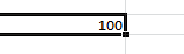
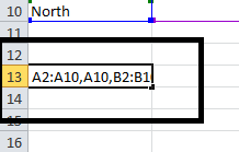
So from the above screenshot, we can quickly determine the total sales incurred in the North Zone, which is "100". Moreover, we can also use the cell reference in the criteria instead of North.

As depicted in the below-attached screenshot.

 After that we should press the enter button to get the desired results.

OUTPUT:

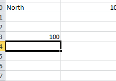
So the total sales for the North Zone are nearly 100, which we get using the A3 as the cell reference.

# Example 4:

We will consider the sales data from the last four months in this example. And we wish to find out the total amount of the sales done for March.

The following data on which we have to perform the operation is depicted below in the attached screenshot.

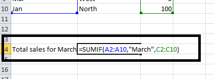
Now, after entering the data for the sales in the other four months. We will now write down the formula in the cell that is B14, which is mentioned below.

• Total sales for March =SUMIF(A2:A10,”Mar”,C2:C10).

As depicted in the figure below.

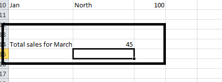
And after that, when we press the "Enter" Button, we will get our desired results. As shown in the below-attached screenshot.

Now we will look forward to some different SUMIF scenarios where the condition or the criteria are in the form of the text, respectively.

#Example 5:

Here, we are considering the simple data related to the flowers and their quantities, as depicted in the attached screenshot below.

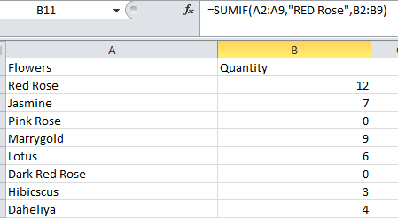
Let us assume that we want to sum up all the red rose flowers, whether it is dark red or pink out of the flowers. Then for that, we will write the formula and then press enter to get the result, as mentioned below, with the help of the screenshot also.

Formula: =SUMIF(A2:A9,"RED Rose",B2:B9)

Things to Remember

The basic as well as the essential things that need to be remembered by an individual while making use of the SUMIF formula in the excel sheet are as follows:

1. First and foremost, this individual should make things a little bit simple to ensure that the range and the sum_range must be of the same or equal in size.
2. And if the condition or the criteria are written in the text, then it should always be enclosed in the double quotes.
3. And an essential thing that needs to be remembered by an individual while working with the SUMIF Formula is that they should not mention the criteria of the text more than 255 characters as it will result in the #VALUE! Error.
4. And in the SUMIF Formula, the sum_range consistently be implemented in the range and not in the form of the arrays.
5. And suppose the case arises where the sum_range is not given. In that case, cells of the range will be added effectively that meet the particular condition or the criteria smoothly without getting any errors.