How to make use of the Wildcard in Excel
In this modern world, it is known that the wildcard characters in Microsoft Excel are considered to be the most essential and unrated features of Microsoft Excel. Besides all these, it was known by most of the public as people in any manner.
Moreover, it is very good to know about the features because it primarily saves lots of the time and effort required to do the same type of research in Microsoft Excel.
And in this article, we will be going out to discover how to use the wildcard characters in Microsoft Excel in brief, with the help of various examples.
What do you meant by the term Wildcard characters?
“Wildcard characters are considered the type of characters present in Microsoft Excel to obtain the result or the outcomes that are primarily less than accurate or exact.”
For example, suppose we have the word “Chat with friends.” So in the database, we have “Chatting with the friends”; then, in that case, the standard letter in these two words is none other than "Friends", so, in these, we can effectively match out with the Excel Wildcards characters in the respective Microsoft Excel.
Types of the Wildcards characters
There are three types of the Wildcards characters that are available in Microsoft Excel are as follows:
- Asterisk (*)
- Question Mark (?)
- Tilde.
And these three wildcard characters primarily have different purposes from each other effectively.
Now moving on to understanding the above three types in detail,
Asterisk (*): It was known that the respective Asterisk primarily represents the number of characters in the following available text string.
For Example, When an individual types Br*, it could mean to be the Broken, Broke, Break. So * after the Br could mean the selection of the only words that usually start with the Break, and it does not matter what type of the words and the number of the characters are after that Br. We can similarly begin the search with the help of the Asterisk (*) efficiently.
Question Mark (?): In the respective Microsoft Excel, the Question marks (?) are used for the single characters.
For Example,? Ove could mean the Dove as well as the Move. So, here is the question mark that primarily represents the single characters M or D effectively.
Tilde: We have already seen that there are two wild characters, Asterisk (*) as well as the Question Mark (?). And the third wildcard character, Tilde, is used to identify the respective wildcard character. Besides these, we have not encountered various situations where we need to use the Tilde, but it's good to know the features in the respective Microsoft Excel.
How to make use of the Wildcard characters in Excel?
Let us click on the examples below to use the wildcard characters in Microsoft Excel effectively.
# Example 1: Filtering the Data with the help of the Wildcard characters
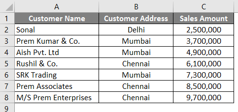
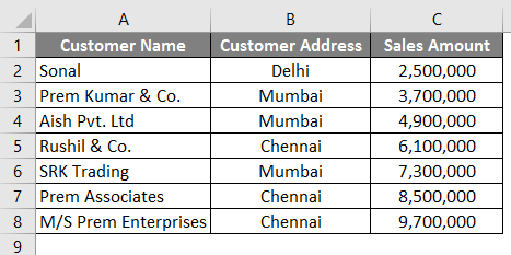
Let us suppose that we are working on the sales data in which we will have the customer's name, address, and sales amount, as clearly depicted in the screenshot below. And in the customer list, we have different companies of the particular parent company, "prem enterprise." So, suppose we need to filter out all the companies associated with the Prem in the customer name. In that case, we will be then just filtering out with one of the Asterisks (*) just behind the Prem and one Asterisk (*) after Prem and will look like "* Prem" and the searching option that will effectively give me the list of all the companies that will have Prem in the company name respectively.
As clearly depicted in the below-attached screenshot respectively,
Now we will follow the below-mentioned steps to do a search and then filter out the companies with the name "Prem" effectively.
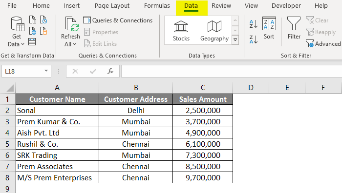
Step 1: First, we will move to the Data Tab in Excel, as seen in the screenshot below.
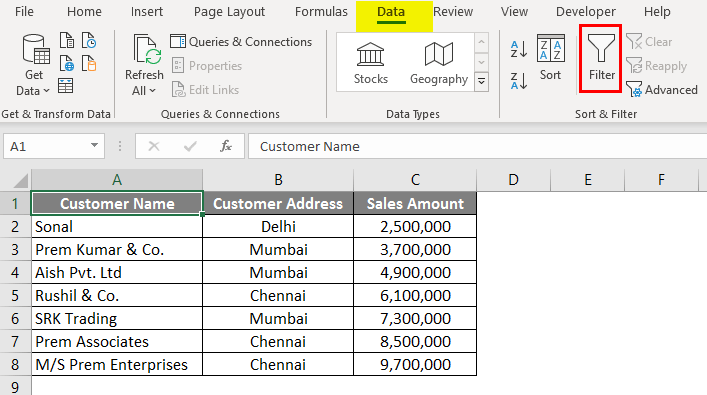
Step 2: Now, after that, we will click on the "Filter Option", as seen in the below-attached screenshot.
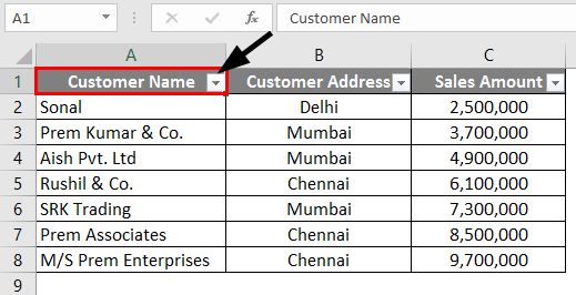
Step 3: Now, once the filter is applied, then move to Column A, which is the "Name of the Customer", and then we will click on the drop-down box as seen in the below-attached screenshot respectively.
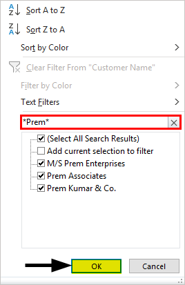
Step 4: And in the particular Search Field, type "*Prem", and then we will click on the "Ok" button, as seen in the below-mentioned figure.
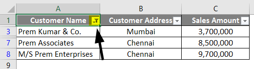
After performing the above steps, we can see that all three respective companies with "Prem" in their name have been filtered and selected efficiently, as shown in the screenshot below.
# Example 2: Finding and Replacing of the words with the help of the Wildcard characters
There can be various areas where we can use the wildcard characters effectively to find and replace the words in the Microsoft Excel sheet. Now, consider the examples we selected in Example 1, as seen in the screenshot below.
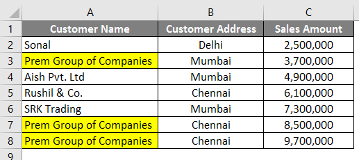
As we can see in the very first example, we have made filtration of the companies name that has "Prem" in their name, so in this particular example, we will now try to find out the companies which have "Prem" in their name and then making out the replacement of the company with the reputation that is none other than the "Prem Group of Companies."
And To do all these, we need to follow the below-mentioned steps one by one.
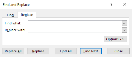
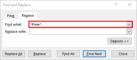
Step 1: Firstly, we will press the shortcut that is CTRL+H in Microsoft Excel, and after performing these steps, we will be encountered the dialogue box, which is seen clearly in the below-attached screenshot.
Step 2: Now, in the Find what field, enter the respective word "* Prem" to make searches of the name of the respective companies with the "Prem" in its name respectively, as clearly depicted in the below-attached screenshot.
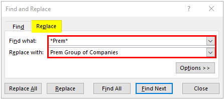
Step 3: After that, in the "Replace with" option, we need to enter the word "Prem Group of Companies." As seen in the below-attached screenshot.
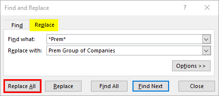
Step 4: In this step, we will now click on the "Replace All" buttons in such a way that it will be replacing out all the names of the respective companies that have "Prem" in its name with the "Prem Group of the companies” as we can see in the below-attached screenshot.
Step 5: After clicking on the particular "Replace All" button, we will effectively get out the below dialogue box, as seen in the below-attached figure.
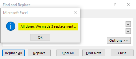
After performing, all the steps mentioned earlier, we can see that the respective companies' names in rows 3, 7, and 8 are changed to the “Prem Group of the Companies.”
As we can see in the below-mentioned steps,
# Example 3: Vlookup with the help of the Wildcards characters in the Excel
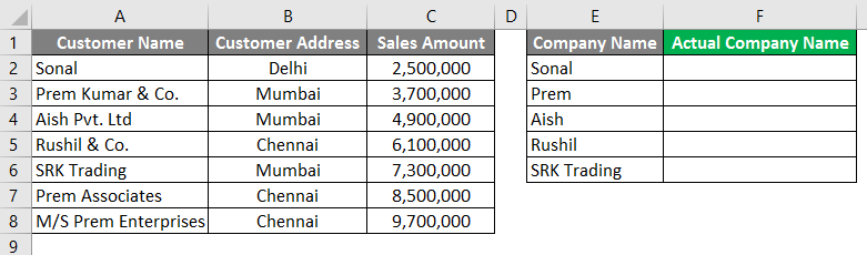
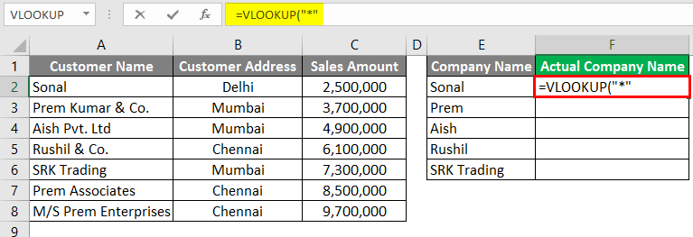
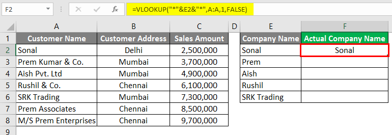
As we have seen in the example mentioned earlier, we have used the Wildcards to find and replace the word in Microsoft Excel. Similarly, we are using the wildcard characters in the particular Microsoft Excel Vlookup. Again, we are taking out the same example as taken for example 1, and besides these, we are adding to the data as assumed in example 1. And for these, we will have the table with the initial reference of the company name as in column E. As we can see in the below-attached screenshot,
It was known that the standard Lookup would be not working hers as the respective names are not similar, as it is seen in the column that is column A and column F. So for these, we need to give a lookup in such a way that it should pick out the result for the same company names as in column A.
Now we are moving further with the below-mentioned steps to see how we can do the following things.
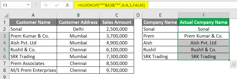
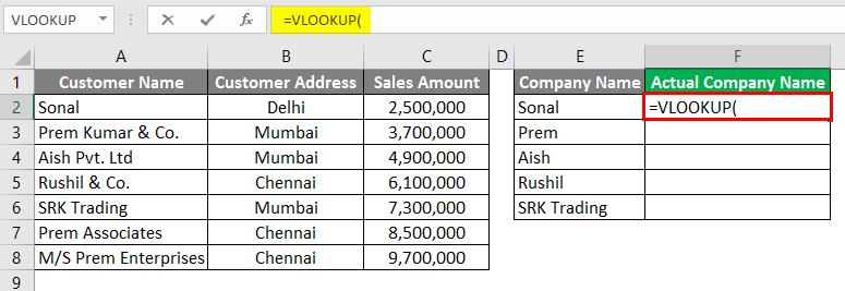
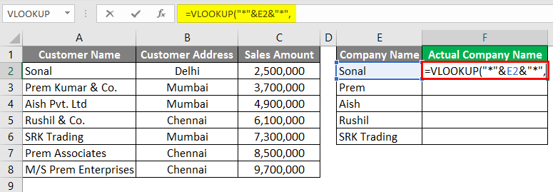
Step 1: Firstly, we will enter the formula for the Vlookup in the particular column, column F2, as clearly depicted in the below-mentioned figure.
Step 2: After that, in these steps, we will start the Vlookup value with the help of the Asterisk (*), as we can see in the below-attached screenshot.
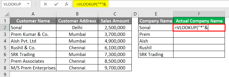
Step 3: Now we will be typing the "&" to connect the reference with the cell that is the E2, as seen in the below-attached screenshot.
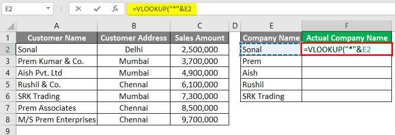
Step 4: In this step, we will be giving out the reference for the individual cell, that is, cell E2, as can be seen effectively in the below-attached screenshot.
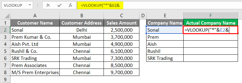
Step 5: Now, after that, we will be again typing the "&" just after the cell reference, as we can see in the below-attached screenshot.
Step 6: In this step, we will send the value of the Vlookup with the help of the Asterisk in between the semicolons "*" as shown in the screenshot below.
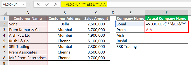
Step 7: Now, for the respective Table_Array in the Vlookup, we will be giving out Columns A's references so that it will effectively pick out the values from Column A, as depicted in the below-attached screenshot.
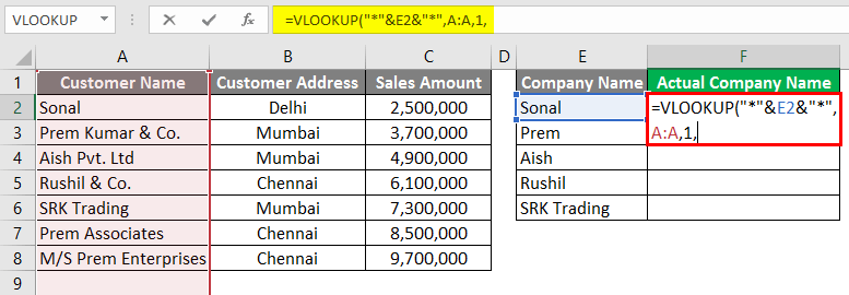
Step 8: Now, in the column index, we can easily select one as we need the value from Column A, as seen in the below-attached screenshot.
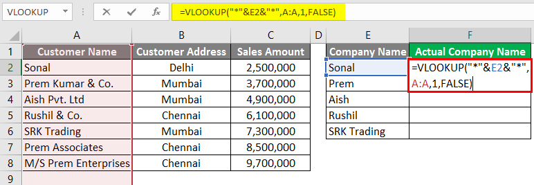
Step 9: In this step, for the last condition in the Vlookup formula, we can easily select FALSE for the exact match efficiently, as is depicted in the below-attached screenshot.
Step 10: After that, we will press the "Enter Key, " as shown in the screenshot below.
Step 11: Now, we will effectively drag down the particular formula to the below-mentioned row and see the result or the outcomes.
Things to Make Remember about the Wildcard in the Microsoft Excel
The important thing that needs to be remembered by an individual while working with the Wildcard in Microsoft Excel is as follows:
- The respective Wildcards characters need to be used carefully because they can be efficient results or outcomes from the other individual options, which can arrive with the help of the same logic.
And for these, we need to check those mentioned options carefully. For example, in particular, example 3, where we have made use of the Lookup with the help of the wild card characters, in which there are three companies with the "Prem" in their name, but we can see that it has been captured only the first company name that has "Prem" in its name in the particular column A effectively. - And the other most crucial thing that needs to be remembered by an individual is that the Wildcards characters can be efficiently used in the various other functions of Microsoft Excel, such as the count functions, Vlookup functions, and the match functions, etc. So, it is known that an individual can effectively use particular wild characters in many innovative ways.
- Besides all these, an individual can also use the combo of the Asterisk (*) and the question marks (?) in some of the conditions and the situations if necessary or required to be performed.