How to use Index and Match in Excel?
The Index and Match function is a familiar and frequently used function in Excel. It is one of the most powerful functions and is easy to use. By default, Excel contains multiple formulas and functions in a default manner, which are used to perform various calculations. Among these functions, the Index and Match function is used to perform the task of various lookups. Lookups include,
Horizontal and vertical lookup
- Two-way lookup
- Left lookup
- Even lookup
- Case sensitive lookup
- Even lookup
The detailed functionality of various lookup is described clearly with an example as follows,
INDEX Function
The INDEX function displays the value at a given location in a range. The steps to be followed to use the Index function is,
Step 1: Enter the data in the respective row or column, A1:D10.
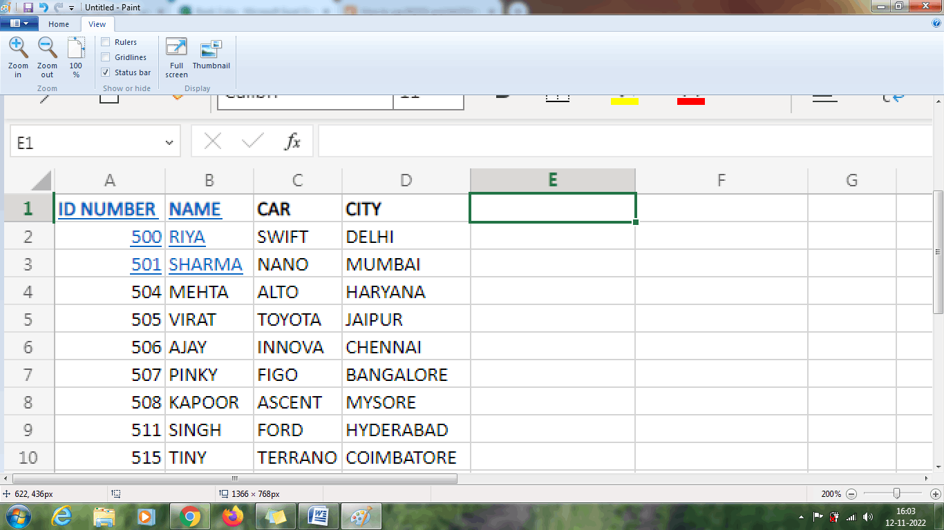
Step 2: Select the new cell where the user wants to display the result, namely E1:F1.
Step 3: In cell E1, type "NAME" and in F1, type the formula as =INDEX (B2:B10, 4). Here '4' indicates the fourth value present in row B2:B10.
Step 4: Press Enter. The result will be displayed as VIRAT in cell F1.
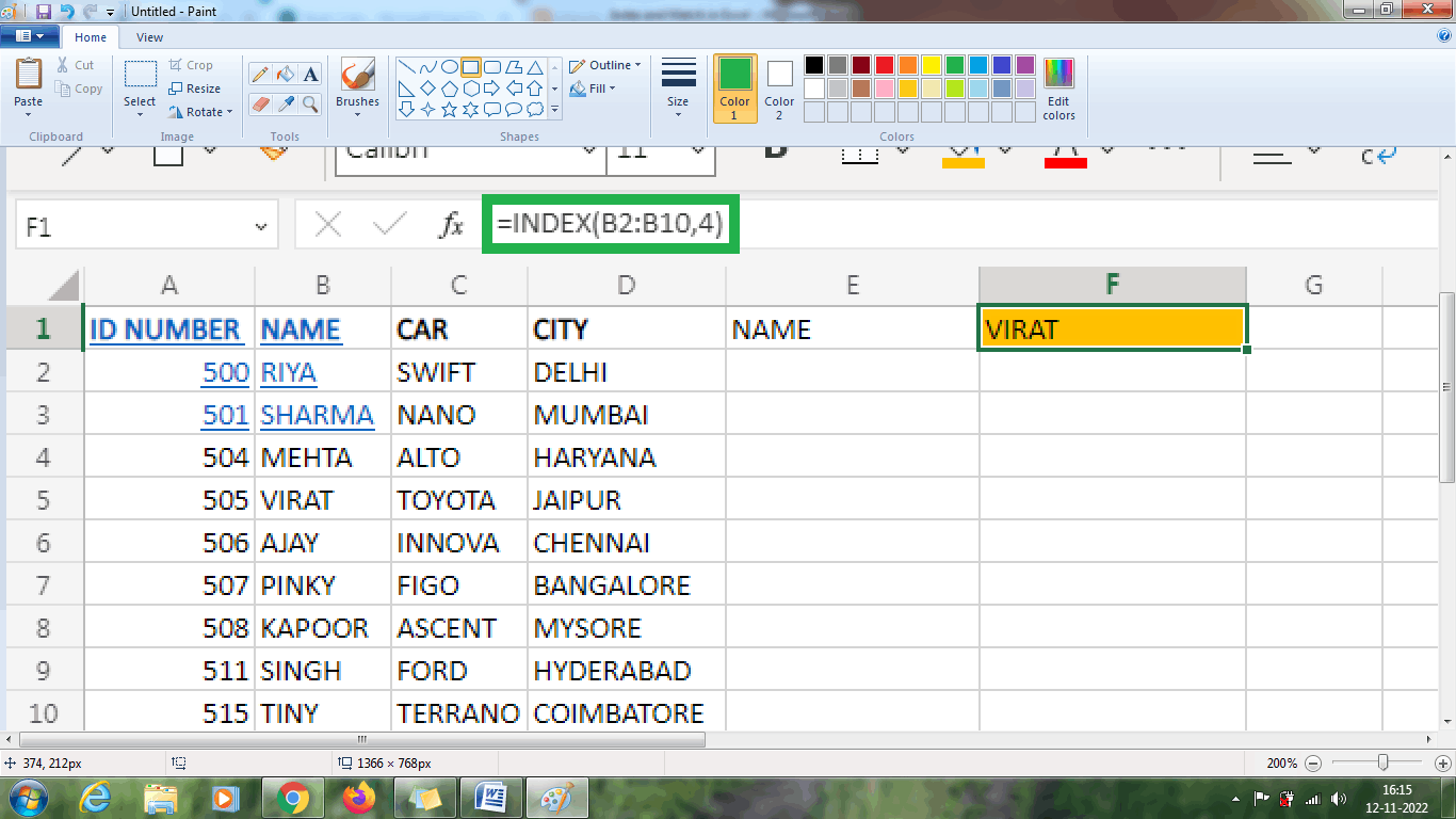
From the above worksheet, the index function returns the value present in cell B5, which is the 4th value in column B2:B10.
Here is another method for the Index function to display the car name as follows,
Step 1: Enter the data in the respective row or column, A1:D10.
Step 2: Select the new cell where the user wants to display the result, namely E1:F1.
Step 3: In cell E1, type "CAR," and in F1, type the formula as =INDEX (B2:C10, 4, 2). Here 4 and 2 represent the data to be displayed, which is present in the fourth row and second column.
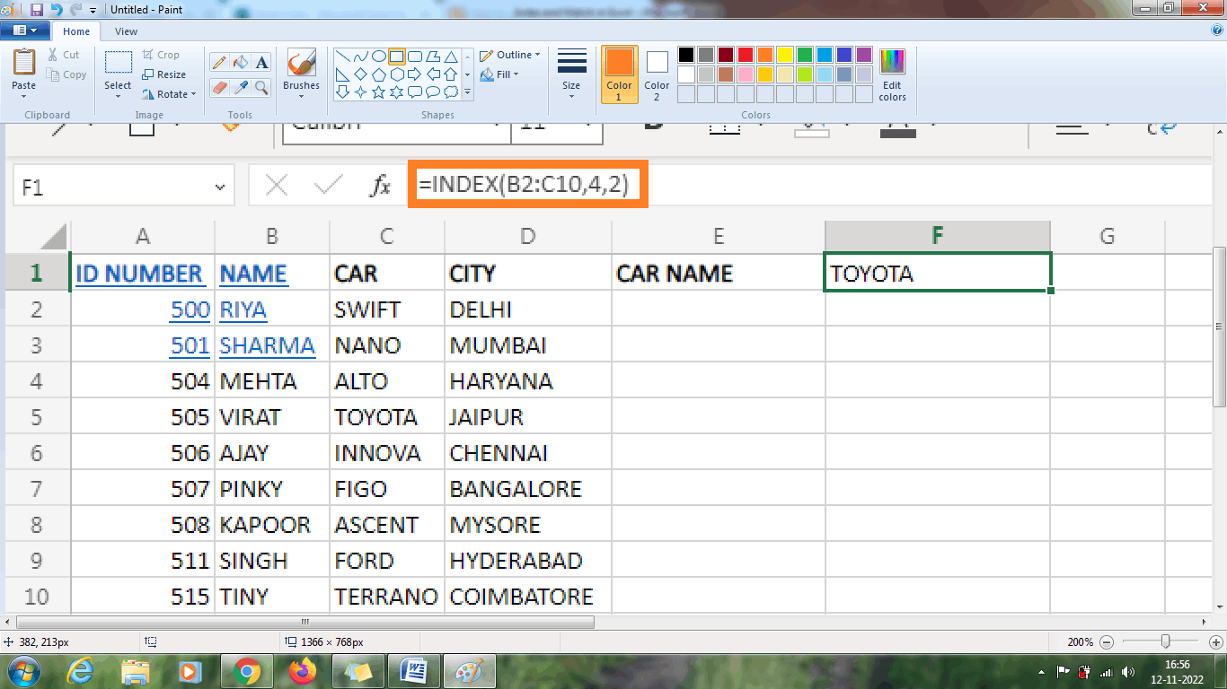
From the above example, "TOYOTA" is displayed, which is present in the 4th row and 2nd column in the data range B2:C10.
MATCH Function
The MATCH function is used to find the position of the given data or value. The steps to be followed to use the MATCH function are as follows,
Step 1: Enter the data in the respective row or column, A1:A10.
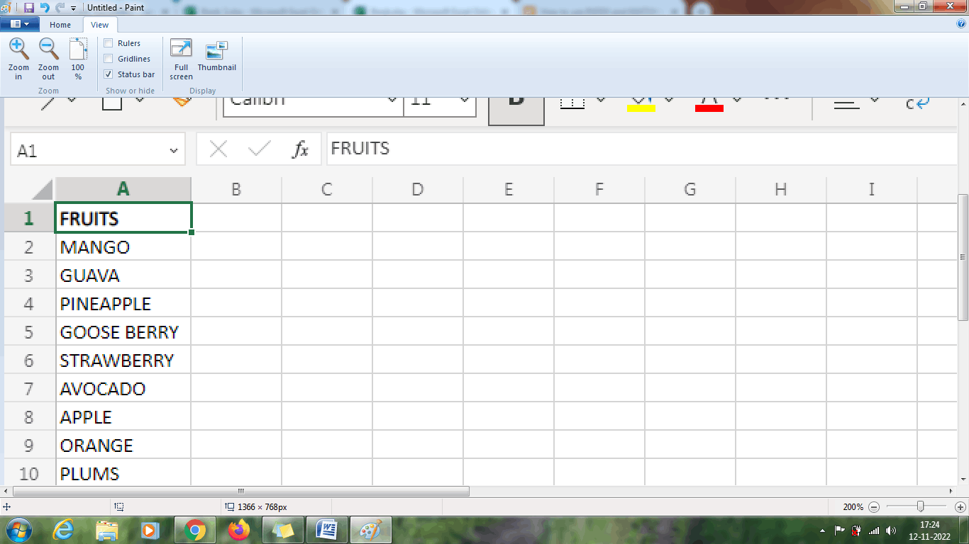
Step 2: Select the new cell where the user wants to display the result, B1:C1.
Step 3: In cell B1, type "Fruit Name," and in C1, type the formula as =MATCH ("Avocado", A2:A10, 0).
Step 4: Press Enter. The formula returns the exact position of the fruit “Avocado”.
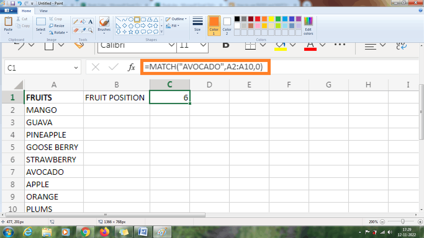
From the above worksheet, the position of the fruit "Avocado" is displayed as "6," which is present in the sixth position of the column range A1:A10.
Here is a method for the MATCH function to display the position name of the data, which is present horizontally or vertically. The steps to be followed are,
Step 1: Enter the data in the horizontal manner row from A1:I1.
Step 2: Select the new cell where the user wants to display the result, namely
B2.
Step 3: In cell A2, type "Fruit Name," and in B2, type the formula as =MATCH (“Avocado”, B1:I1, 0).
Step 4: Press Enter. The formula returns the exact position of the fruit "Avocado," where the data are presented horizontally.
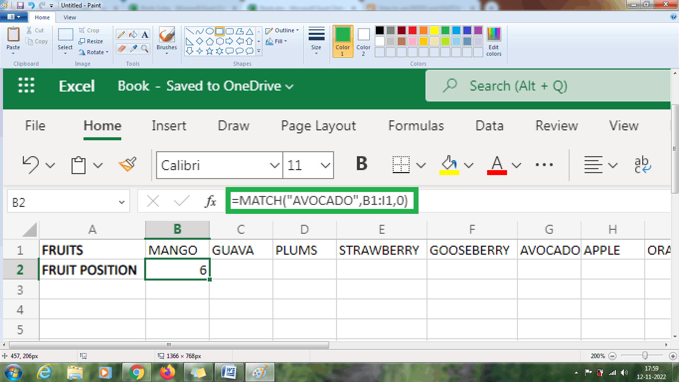
The above worksheet displays the result as "6," which is the position of the fruit Avocado horizontally.
Combination of INDEX and Match Function
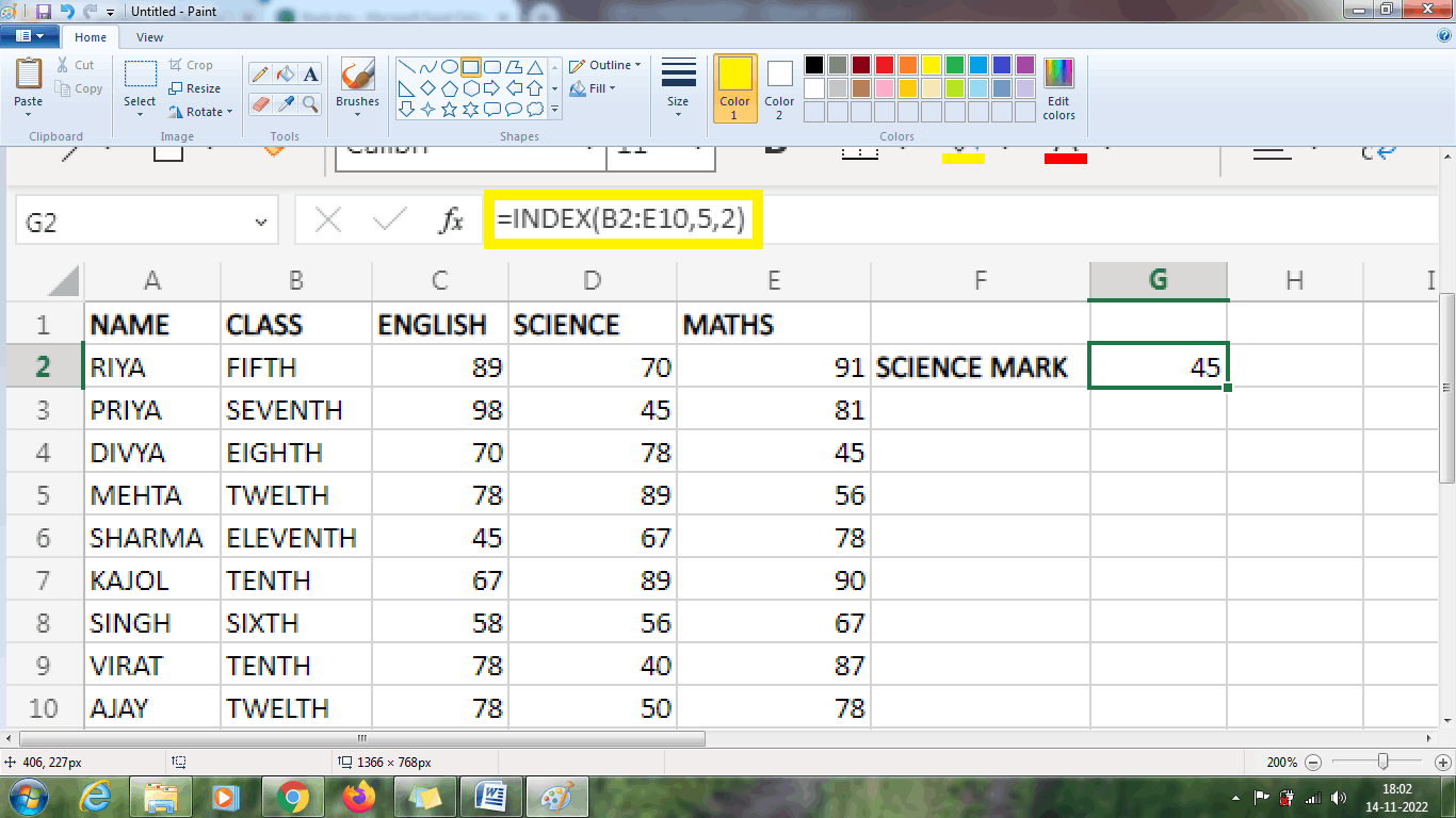
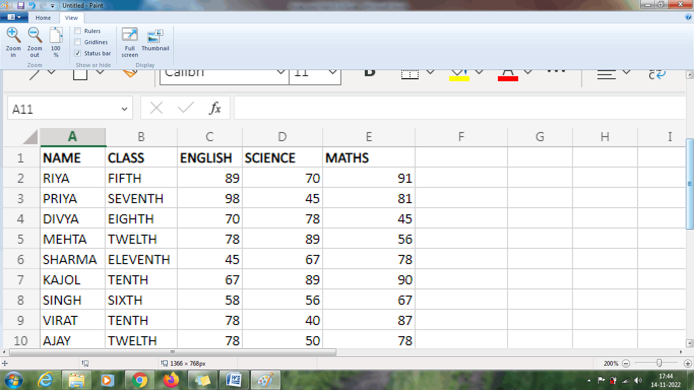
Here, in this example, the combination of INDEX and MATCH functions is used to retrieve the values. For example, the marks of various students in the same class for the respective subjects are shown below.
Step 1: Enter the data in the respective row and column, namely A1:E10

From the above data, to find the ENGLISH Mark for SHARMA, the steps to be followed are as follows,
Step 2: Select a new cell, namely G1, and enter the formula as
=INDEX (B2:E10, 5, 2)
The above INDEX formula helps to retrieve the data from the respective row and column. Here the value is retrieved from the 5th row and 2nd column.
The MATCH function is nested inside the INDEX function to implement the dynamic lookup.
The formula for dynamic lookup is =INDEX (B2:E10, MATCH (“SHARMA”, A2:A10, 0), 2). The MATCH function finds the exact position of the required data.
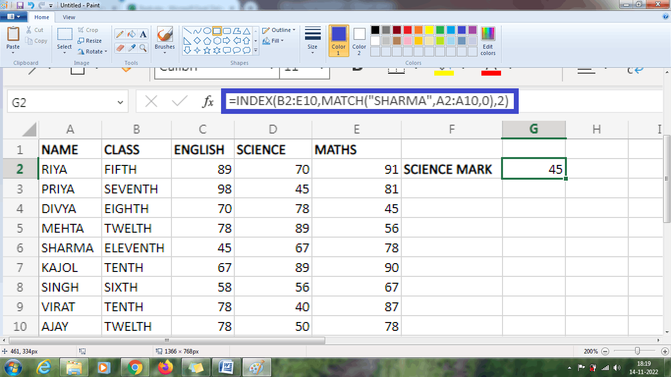
From the above worksheet, the MATCH and INDEX functions find the exact data in the position.
An alternative method to find the position of the data in the given table, the formula used is,
=INDEX (B2:E10, MATCH (G2, A2:A10, 0), 2). Here G2 is the cell where the Name “Sharma” is present. To display the exact data present in the mentioned row and column, the steps to be followed are,
1. Select a new cell, G2, and type SHARMA.
2. Enter the formula as =INDEX (B2:E10, MATCH (G2, A2:A10, 0), 2) in the cell G3.
3. The result will be displayed in cell G3 as 45, the English mark of Sharma.
Two-way lookup
The above concept identifies the row number dynamically, but the column is hard coded. To make it fully dynamic, the MATCH function is used twice to retrieve the row position once and the column position once.
Here in this method, using INDEX and MATCH functions, a two-way lookup is used to find the respective data.
As is already known, the MATCH function works with horizontal and vertical arrays. For example,
=MATCH (“ENGLISH”, A1:E1, 0)
The MATCH function returns the position as 3. But here, the value "ENGLISH" is hard coded. To use the function without hard coding any values in the formula, the steps to be followed are,
Step 1: Enter the data in the respective row and column, namely A1:E10
Step 2: To find the Math mark for Sharma, in cell G1, enter "Sharma," and in G2, enter "MATHS".
Step 3: In the cell G3, enter the formula as =INDEX (A2:E10, MATCH (G1, A2:A10, 0), MATCH (G2, A1:E1, 0))
Step 4: The result will be displayed as 78, a Math mark of Sharma.
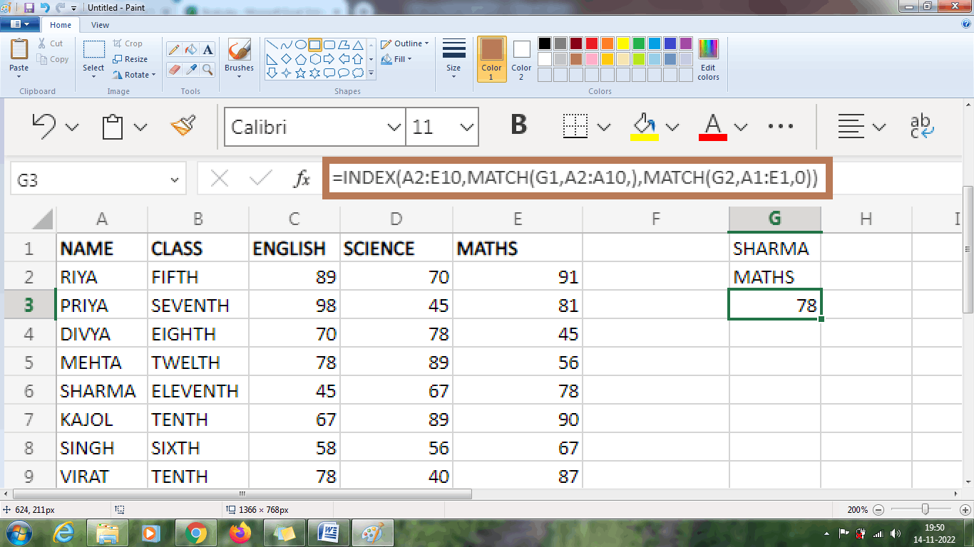
The above worksheet shows the MATH mark of Sharma as 78 using a two-way lookup.
From the above formula, the first Match function indicates the 5th row, and the second Match function indicates the 5th column. Once the MATCH function runs, the formula is simplified as follows,
=INDEX (A2:E10, 5, 5), which displays the result present in the respective rows and columns.
Left Lookup
To perform a Left lookup, the Id number is at the right of the table where the required values are retrieved. The steps to be performed for the left lookup are as follows,
Step 1: Enter the data in the respective row and columns
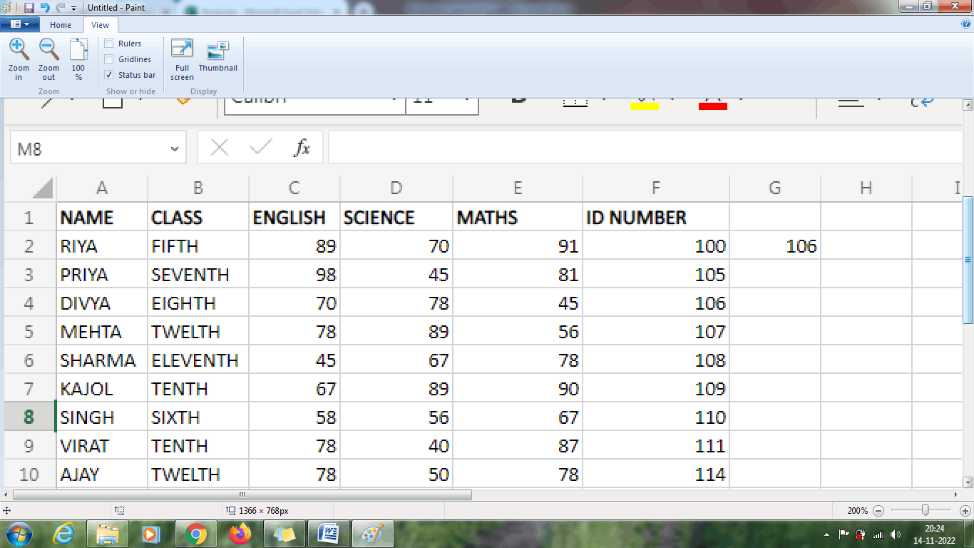
Step 2: To display the name Divya using left lookup, select a new cell.
H2 and enter the ID number as 106.
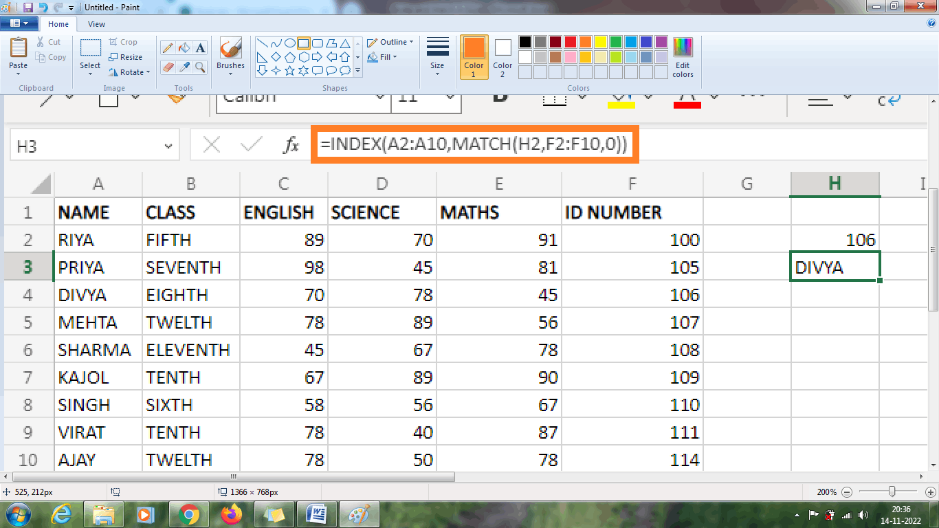
Step 3: Select a new cell where the user wants to display the result, namely H3, and enter the formula as =INDEX (A2:A10, MATCH (H2, F2:F10, 0))
Step 4: The result will be displayed as DIVYA in cell H3.
Case Sensitive Lookup
The Match Function is not case-sensitive. Combining the EXACT function with the INDEX and MATCH functions looks for both lower and upper case. The steps to perform Case Sensitive Lookup is as follows,
Step 1: Enter the data in the respective row and column.
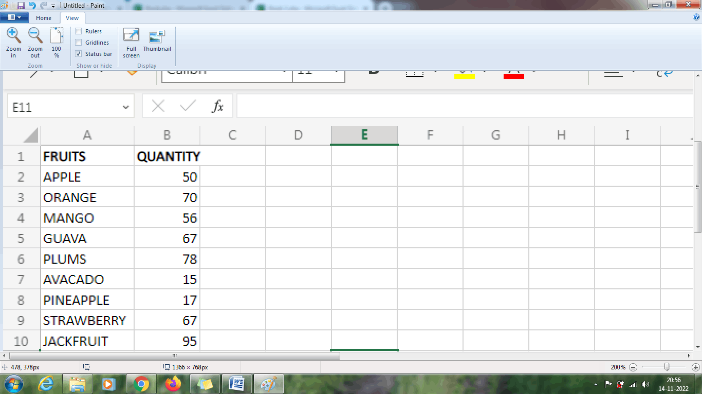
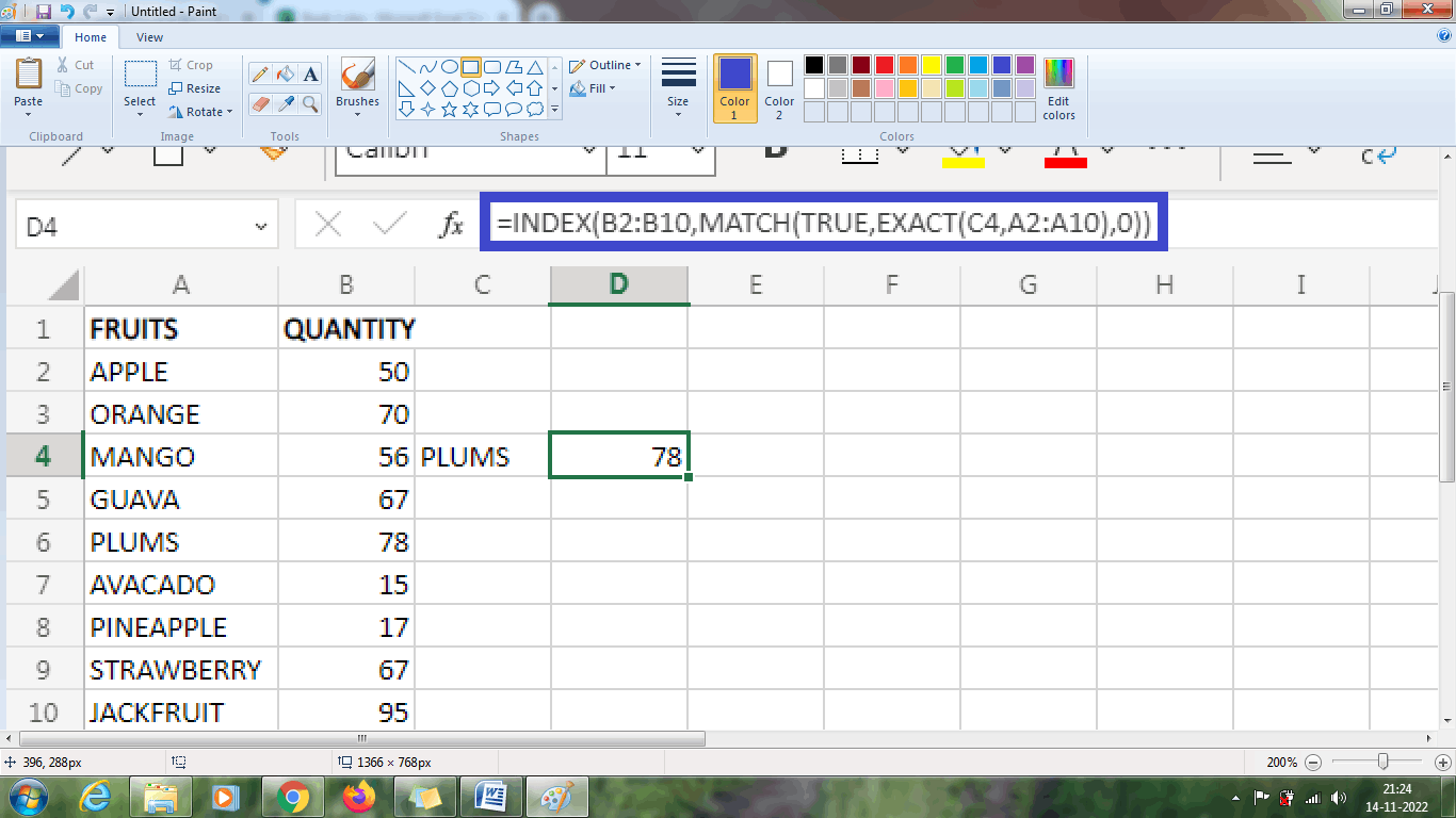
Step 2: To display the quantity of the fruit Plums, select a new cell, namely C4 and enter the fruit name as Plums.
Step 3: Select a new cell where the user wants to display the result, namely D4, and enter the formula as =INDEX (B2:B10, MATCH (TRUE, EXACT (C4, A2:A10), 0))
Step 4: The result will be displayed in cell D4 as 78, which is the number of PLUMS.
Summary
From the above tutorial, the various functions and methods of using INDEX and MATCH are explained clearly.