Data analysis is a powerful tool that helps the users to make better decisions by comparing different information. Microsoft Excel extends its credibility to enforce the data analysis tool and, thus, is one of the most popular analytics tools. This tool is used to aggregate data and visualize useful data. Following are the features that make the data analysis possible in Excel:

What-If Analysis?

Suppose you have a cell A10 which is formula driven i.e. has a formula and the formula is based on values in different cells (A1, A2, A3, A4), what-if analysis helps us in understanding the changes to A10 when values in cells A1, A2, A3 or A4 are altered.

Using the following steps, you can incorporate ‘What-if Analysis’ in your work –

Go to Data Tab and click on What-if Analysis and then select Scenario Manager
Click on Add and a new pop-up will appear – put a Scenario name such that you can easily understand what it stands for
Next is changing cells i.e. which cells you want to change to see the impact
I have put Scenario Name as DP 20% which is current scenario
In ‘Add Scenario’ – I select the cell consisting of the value corresponding to Down Payment
And click on OK – a prompt will appear in which excel asks for the value you want to see – currently it is 0.2 – click on OK
Add 2 more scenarios DP 30% and DP 40% following the same process and corresponding values will be 0.3 and 0.4 and then click on OK
Now you can see 3 different scenarios – you can select anyone and see the difference it leads to the 4 values ‘Loan Amount’, ‘Monthly Payments’, ‘Total Interest’ and ‘Total Payments’

Now what if you want to see the impact of these changes to Down Payments in one table itself side-by-side? For this, we will introduce a new functionality ‘Data Tables’.

What is a Data Table?

A data-table represents the range of cells that provides the values of cells (driven with formula) with respect to the change in values in input cells are changed. In our example, input cells are Purchase Price, Down payment, Loan Term and Interest Rate.

Goal Seek

Goal seeking is used when you have a value in mind for your dependent variable (which is formula based) and you want to change the value of one input variable to achieve that value.

What if in the previous example where ABC bought a car had in his mind that he will not be paying more than $1,400 instalment per month – to achieve this, either he will buy a car which is less costly or he will pay more down-payment or he will increase the term of the loan or he will look for a better deal on the interest rates.

Let’s say ABC is comfortable with price of the car, loan term and interest rate being offered on the loan but wants to change the down payment so that he

can have a monthly EMI payment of $1,200 –

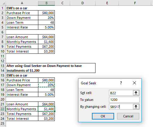
Go to ‘Goal Seek’ by clicking on ‘What-If Analysis’
A ‘Goal Seek’ prompt pops-up – first section from Row 1 to Row 10 has been kept for easy reference to see the different after using ‘Goal Seek’
Since we want to change ‘Monthly Payments’ to $1,200 from current $1,400, we select B22 in ‘Set Cell’ and mention 1200 in ‘To Value’
Since we want to change the down-payment only, we select B17 and click on ‘OK’

The results are shown in picture below. You can compare the top 2 tables with the below 2 tables to see the change due to ‘Goal Seek’ -

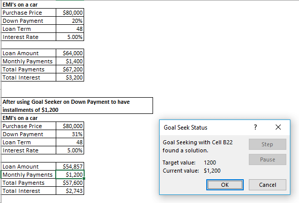
Because ABC wanted an EMI of $1,200, keeping purchase price, loan term and interest rate constant, Goal Seeking has changed Down Payment to 31% from previous 20%.

Analysis ToolPak

How to install Analysis ToolPak? And what is it?

If Analysis tool pack is not installed by default, then –

Go to File (or click on Window’s icon next to Home in the Toolbar’
Click on it and then click on ‘Options’
Now click on ‘Add-Ins’ and then click on ‘Analysis ToolPak’ and click on ‘OK’
A new section ‘Analyze’ will appear in ‘Data’ tab of the toolbar

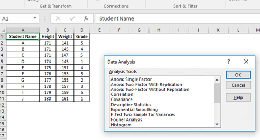
On clicking on ‘Data Analysis’, you will get a pop-up showing different options which you can use to analyse your data or perform statistical tests on your data.

Descriptive Statistics

Thisoption gives different summary statistics likeMean, Median, Mode, Standard Error, Standard Deviation, Variance, Sum, Count – variables which give information about the kind of data we have in our dataset.

To use this tool, once you have selected ‘Descriptive Statistics’ option, a pop-up will appear as shown in the picture below –

Since I want descriptive statistics for all the 3 variables (numeric variables) in my dataset, in the input range I have given their location
Since the first row consists of ‘Column Headers’ i.e. column names, I do a tick for ‘Labels in first row’ option
I want my metrics to be given on a new worksheet, so I have selected that option – I can also output the results in a different workbook
I have checked last 4 options to get summary statistics – for the ‘Kth largest’ and ‘Kth Smallest’ options I have given values 2 and 3 because I want to know the 2^nd largest and 3^rd smallest value – you can change this as per your liking but cannot be more than the number of observations/rows in your dataset
Click on OK

Analysis of Variance

Also known as ANOVA, determines whether two or more samples were drawn from the same population or not by taking their mean into account. The null hypothesis is that the 3 samples are not statistically different i.e.

H0: µ1 = µ2 = µ3 …… = µk

If the results come statistically significant, we accept the alternate hypothesis H1 that at least 2 samples are different i.e. if F Calculated is greater than F Tabulated, then we reject null hypothesis.

t-Test

t-test is used to test the null hypothesis that the means of two populations are same. This test is used when the number of observations in our samples or population is less than 30 – greater than 30, we usually use z-test then.

There are 3 types of t-tests in Excel –

Paired Two Sample for Means i.e. when the population or sample on which the test is being done is same for ex: marks obtained by a group of 10 students before maths coaching class and after taking maths coaching class i.e. the sample population is the same 10 students just that their performance is being compared before and after an event
Two-Sample assuming Equal variance i.e. when the samples are different (independent of each other) – 2 groups of 10 students being compared with excel assuming equal variance
Two-Sample assuming Unequal Variance - same as above just that variance is either unknown or different
Null hypothesis can be that the mean of the 2 samples is same in which case it is a two-tailed test. For a one tailed test, null hypothesis can be µ1 > µ2 or µ1 < µ2 with the alternate hypothesis being that the means are different.

H0: µ1 = µ2

H1: µ1 ? µ2

Solver

The Solver feature is used when the user wants to maximise or minimize the dependent value of predefined dependent variable (which is formula based) and you want to change the values of the input variables to achieve that value. It is the reverse of the ‘What-If Analysis’.

Below are the steps to use Solver –

Enter the data in the excel sheet and click on the ‘Data’ tab
Select the ‘Solver’ option in the ‘Analyze’ section
In the ‘Set Objective’ option select the cell that you would like to minimize, maximize or set to a value
In ‘By Changing Variable Cells’, you will have to enter all the input cells which you want to be changed
For ‘Subject to Constraints’, we can add constraints like overall production of the facility is less than a number 450 or each product production needs to be above a specified limit
Click on ‘Solve’ option and excel will display the results but if it won’t be able to meet all the constraints, it will display a prompt dialogue box with the same message.

Histogram

The Histogram tool is useful for producing data distributions and histogram charts. It accepts an

Input range and a Bin range. A bin range is a range of values that specifies the limits for each column

of the histogram. If you omit the Bin range, Excel creates 10 equal-interval bins for you.

The size of each bin is determined by the following formula:

=(MAX(input_range)– MIN(input_range))/10

If you specify the Pareto (Sorted Histogram) option, the bin range must contain values and can’t

contain formulas. If formulas appear in the bin range, Excel doesn’t sort properly, and your worksheet

displays error values. The Histogram tool doesn’t use formulas, so if you change any of the

input data, you need to repeat the histogram procedure to update the results.

Excel Tutorial

Functions

How To

Misc