
Purpose of Randomize in Excel
Excel spreadsheets are used on a large scale for business and personal usage. It is used to store data, perform multiple calculations, make assumptions based on charts and graphs etc. Coming to the concept of randomized data, Excel generates random numbers. Random numbers act as an input to the formula to check multiple results and determine whether it works under various conditions.
It is used to sort the actual data, assign different values to the other person, and process multiple customer requests in random order. Excel provides a default random number generator called RAND, a built-in function used in a formula. It generates the random real number between zero and one.
What is Randomize List?
The term Randomize is also known as shuffle in general English. Its function is used to shuffle the data in the list using RAND function and SORT function. The purpose of RAND function is to shuffle the data randomly and sort is used to sort the data.
The syntax for the formula is “=RAND()” which generates the random number. For example to generate a random number between two variables namely “x and y”, the formula used are “=RAND()(y-x)+x”. To generate a whole number use INT function called integer which takes the integer part of the decimal number.
Syntax for the formula be “=INT(RAND()(y-x)+x)”. If the values present in the sheet are recalculated, the new random data will be generated.
RANDBETWEEN() Function
The RANDBETWEEN function is used to execute the random numbers between two various boundary numbers. For example, “=RANDBETWEEN (1, 10)” will execute the random integer number 1 and 10. This function is used to generate the random numbers for simulations, games of chance and raffles.
A simple method is to insert random numbers for all columns, just insert the formula in the particular cell and drag the + sign to insert the formula downward. This will help to insert the random numbers in all columns.
Random Sort
Random sort function helps to sort the randomized data present in the rows or columns. After inserting the RAND () formula in the cell, the randomized data are present in all the cells. To sort the randomized data just, click the “Data” tab and choose the option called “Sort A to Z” to sort the data present in the cells. After sorting the user are allowed to hide the randomized data present in the cell.
What are the various methods to randomize data in Excel?
There are five different methods to randomize the data present in Excel.
- RAND Formula
- RANDBETWEEN Formula
- RANDARRAY, SORTBY and ROWS Formula
- INDEX and RANDBETWEEN formulas
- CHOOSE and RANDBETWEEN formulas
1. How to use RAND() formula?
Step 1: Enter the set of data in the respective column namely A1:A5
Step 2: Select the cell B1 which is next to the cell A1 and insert the formula as =RAND ().

Step 3: If you wish to insert the randomized data to all the remaining columns, click the “+” sign and drag towards cell A5. The respective cell is inserted with randomised data.

How to apply SORT() function?
In the above chart randomized data are present in the data table. To sort this data, choose Sort and Filter data in Data tab.

Do you know you can sort the above data in ascending order as well. Go to Sort & Filter-> Click on Sort Ascending.

The sorted data are list are as follows,

Usually the random numbers change every time in the spreadsheet, hence if it is needed copy and paste it in the new location for future reference.
How to use RANDARRAY() function?
The RANDARRAY function generates a list of random decimal numbers between 0 and 1. The steps to be followed to insert a RANDARRAY function are as follows,
Step 1: Insert the data in the spreadsheet. Here the data are entered in cell range A1:A5
Step 2: Select cell B1 and enter the formula as =RANDARRAY (5, 1).HERE number ‘5’ denotes the number of columns, and the number ‘1’ represents the row.
STEP 3: The result will be displayed in the cell range B1:B5 as follows,

Here the RANDARRAY function fills the value in multiple cells at a time. This process is called spilling.
RANDARRAY and SORTBY
Here the SORTBY function is used to sort the values, which sort the data in ascending order in a default manner.
Step 1: Select the cell range A1:A5 and B1:B5 simultaneously to apply the SORTBY function.
Step 2: Select the new cell to display the new data. Enter the formula as =SORTBY (A1:A5,B1:B5). This sorts the data as shown in the image as follows,

RANDARRAY, SORTBY and ROWS
Row function is used to count the number of rows in the number. To implement Row function steps to be followed are,
Step 1: Enter the data in the spreadsheet.
Step 2: After inserting the RANDARRAY and SORTBY function, add the ROWS function.
Step 3: Enter the formula as =SORTBY(A1:A8,RANDARRAY(ROWS(A1:A8),1)
Step 4: The data will be look like below as follows,

Here the functions are used in the formula as SORTBY, RANDARRAY and ROWS.
How to use RANDBETWEEN() function?
RANDBETWEEN function returns a random integer number between the numbers described. Every time a new random number is generated, the calculations are performed on a worksheet. The syntax for this function is,
RANDBETWEEN(bottom, top)
Bottom – It represents the integer value which is smaller in value
Top – It represents the integer value which is larger in value.
To implement this function steps to be followed are,
Step 1: Enter the data in the spreadsheet.
Step 2: Select a new cell range and enter the formula as =RANDBETWEEN(top,bottom)

From the above table the values present in B1:B8 are in the range between (1,100).
How to use INDEX() function?
The INDEX function is used to return the value of the cell or reference to a value from the set of data range or table. The index form is subdivided into two types namely,
Array form – It returns the value of the cell which is specified or array of cells.
Reference form- It returns the reference of the specified cell.
Array form
The syntax of the array form is,
INDEX(array, row_num[column_num])
From the above syntax, this function returns the value of the element from the selected cell which is an array or table format.
Parameters
Array – It represents the cell range or array constant.
If the user’s data contains only one row or one column, then the row or column number is optional. If the data contains more than one row or columns, only the row number and column number is used for representation
INDEX – It represents the complete row or column in an array.
Row number – This function is used to select the entire row which returns a value
Column number – This function is used to select the entire column which returns a value. If row number is not present in the function, column number should present. If column number is not present row number should present.
Let’s have a look, how to use the INDEX function in following methods.
Step 1: Enter the data in the spreadsheet
Step 2: Select a new cell called B1 and enter the formula as =INDEX(CELL RANGE,3,2). Here 3,2 is the intersection of third row and second column.
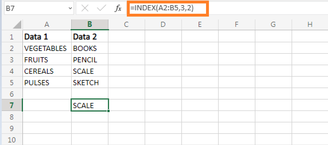
From the above worksheet, the scale option is selected where it is represented using the formula =INDEX(A2:B5,3,2) where 3,2 represents third row and second column.
Using array function for two cells
The INDEX function is used to find the value in two cells which is represented in the form of 2x2 array.
To implement this array,following steps should be followed.
Step 1: Choose a cell name as B1 and enter the formula as =INDEX({3,7;2,5},0,2)

From the above formula, the number 3 and 7 present in the first row and second column where 2 and 5 present in second row and second column.
The resultant value of 7 represnets the first column and second column, where 5 represents the second row and second column.
Reference Form
The Reference form is used to return the reference of the cell which the intersection of respective row and column.
Syntax
The syntax for the reference form is shown below,
INDEX(reference, row_num,[column_num],[area_num])
To implement reference form, following methods are used,
Step 1: Enter the data in the respective row and column wise as shown below,

Step 2: Select a new cell and enter the formula like,
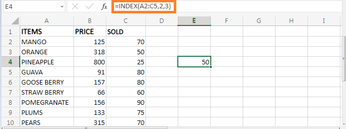
=INDEX(A2:C5,2,3)
A2:C5 is the cell range where 2,3 is the intersection of second row and third column.
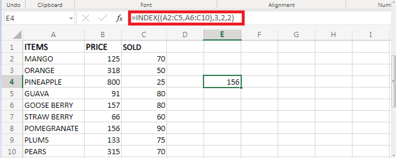
Next enter the formula as, =INDEX((A1:C5,A6:C10),3,2,2)
Here two various ranges are selected in a single table as A1:C5 and A6:C10. The number 3,2,2 denotes the third row ,second column in the second area of A6:C10 which is the cell name of B8.
From the above chart, the result is displayed as 156 which is the value of the cell B8.
How to sum the rows or columns in Excel?
To sum the rows or columns or excel, following steps are followed.
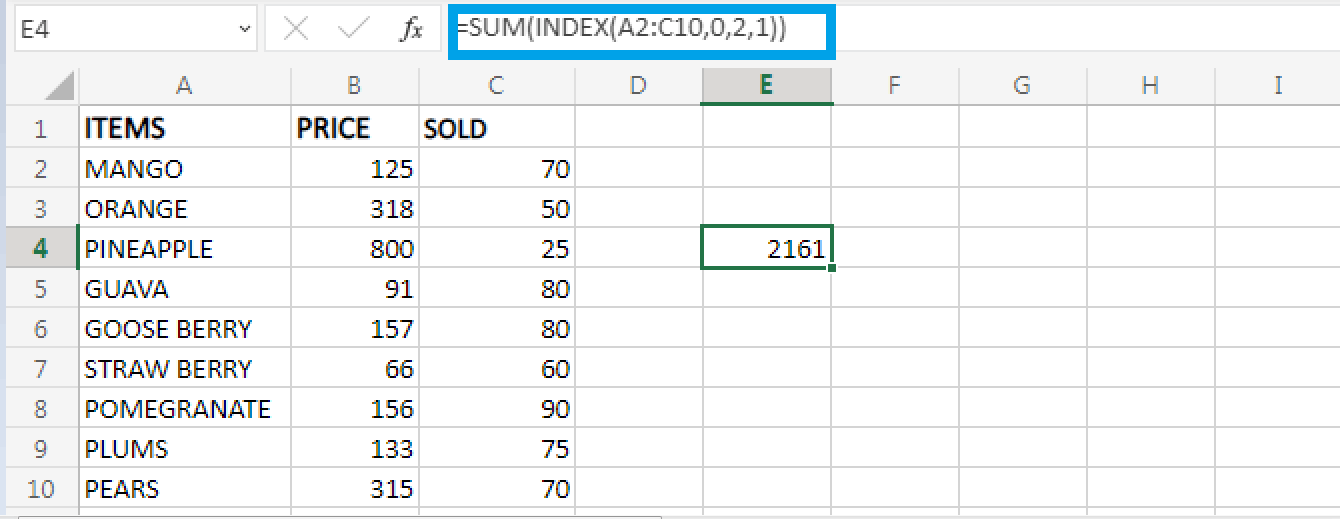
Step 1: Enter the data in the worksheet and select a new cell and enter the formula as =SUM (INDEX (A2:C10,1,2,1)
Here A2:C10 is called cell range. 0,2,1 denotes the second column in the first area.
Here from the above spreadsheet, the result is 2161 which is the sum of the column of B2:B10.
How to implement Choose Function in Excel?
Choose function is used to return a value from a list based on the position.
The syntax for choose function is
=CHOOSE (index_num, value 1,[value 2],…)
Parameters
- Index_num – The number between 1 and 254 is chosen for the value.
- Value 1 – The first value to be chosen.
- Value 2- The second value to be chosen.
To implement choose function, following steps are followed.
Step 1: Enter the data in the spreadsheet as follows.
Step 2: Select a new cell and enter the formula =CHOOSE (2, A1,A2,A3,A4,A5). Here A1,A2,A3,A4,A5 is the cell range where ‘2’ is the index number.

From the above spreadsheet, the value present in the cell A3 is displayed as result where the index number is ‘2’ from the cell range A1:A5.
Summary
From the above tutorial, the various functions and formulas for Randomization is briefly explained.